3 MCDA
3.1 Attributes and Layers
Based on the criteria that we decided to tackle, we had to come up with numerical indicators that we could use to evaluate them. These numerical indicators are called attributes and have to be normalised—in our case between 0 and 1—so that they can be compared and weighted properly depending on their relevance. In our case, 0 corresponds to an urgent need to perform urban stream restoration, while 1 corresponds to a situation that is currently very good, or at least the best in the area of interest.
In practice, these attributes also needed to be aggregable at the scale of the spatial units, so that we can assign one unique value to each spatial unit for each attribute. This can be an important limitation on the type of computations and therefore the type of attributes that we can use. We explain below the different attributes that we computed, how we computed them, which data we used and why we made these choices.
3.1.1 Biodiversity
3.1.1.1 Green-blue connectivity
The aim to measure the blue-green connectivity was to identify the potential areas which can become green corridors along the lengths of the stream. To do that, the area of the vegetation layer from OpenStreetMap was quantified. The layer includes different types of green infrastructure found throughout Dresden, encompassing both designed recreational areas—such as parks and greenery along roads—and natural environments like forests, meadows, and grasslands.
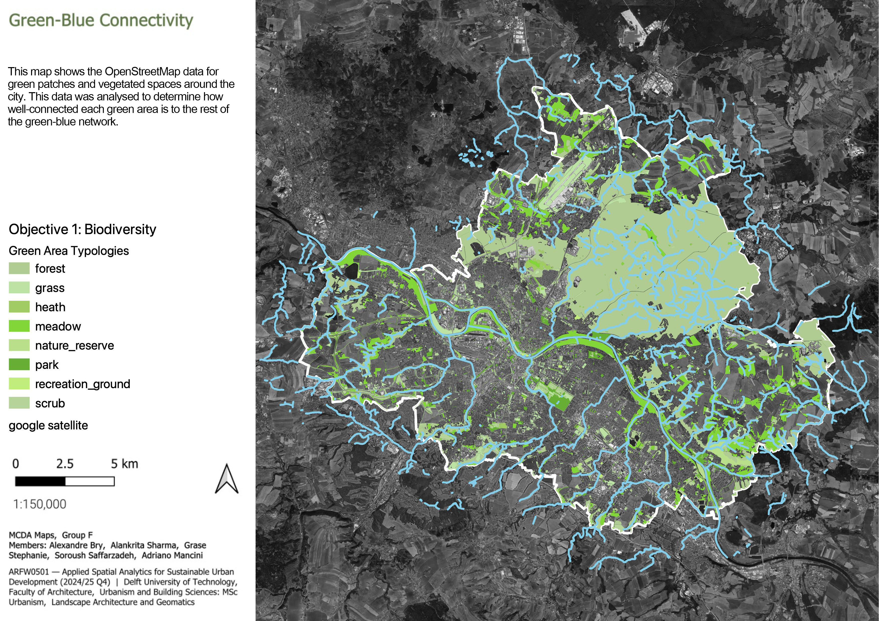
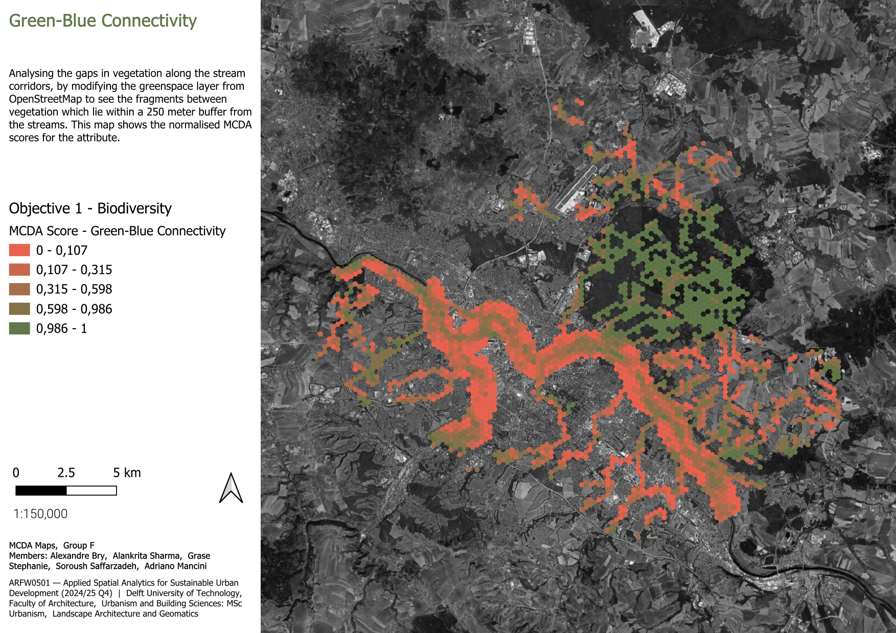
This layer was then intersected with the spatial units to focus on the vegetation which is within a 250m radius from the streams and falls within the defined spatial units. The values of the areas were then graduated to visualise the spatial units which lacked vegetation to those which were densely vegetated. These values were then normalised from 0 to 1 to make them comparable to other attributes. Here, 0 indicates the spaces which lack vegetation and 1 indicates dense vegetation, signalling at the potential spaces to add vegetation and form green corridors along the streams.
3.1.1.2 Soil quality
Soil quality is measured as it is an integral measure of the ecological value of the soil. It is used to understand which areas near the stream have a higher concentration of poor soil quality, as soil health directly relates to the growth of biodiversity. It measured using the Bodenqualität (soil quality) layer from the Dresden open data portal. Soil quality near the streams is visualised by creating a 250 m buffer from the streams and intersecting it with the soil quality layer.
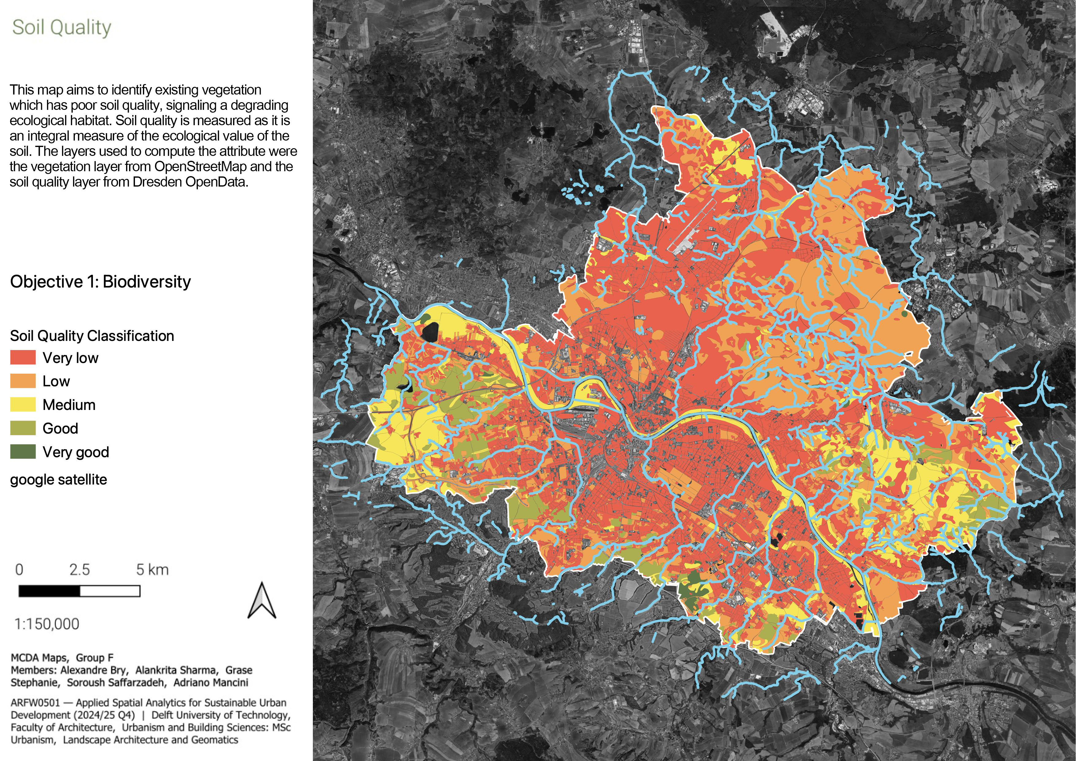
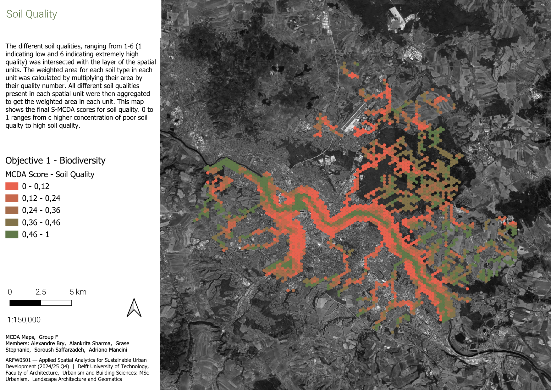
The different soil qualities, ranging from 1-6 (1 indicating low and 6 indicating extremely high quality) was intersected with the layer of the spatial units. The weighted area for each soil type in each unit was calculated by multiplying their area by their quality number. All different soil qualities present in each spatial unit were then aggregated to get the weighted area in each unit. These values were ultimately normalised and graduated to create the final map, which showed us the spatial units where there is a high concentration of poor soil quality, which are necessary to be addressed for biodiversity. Few spatial units do not have any value, aa the layer did not hold any data at those locations. Those units are dropped out from the MCDA analysis.
3.1.1.3 Plant health
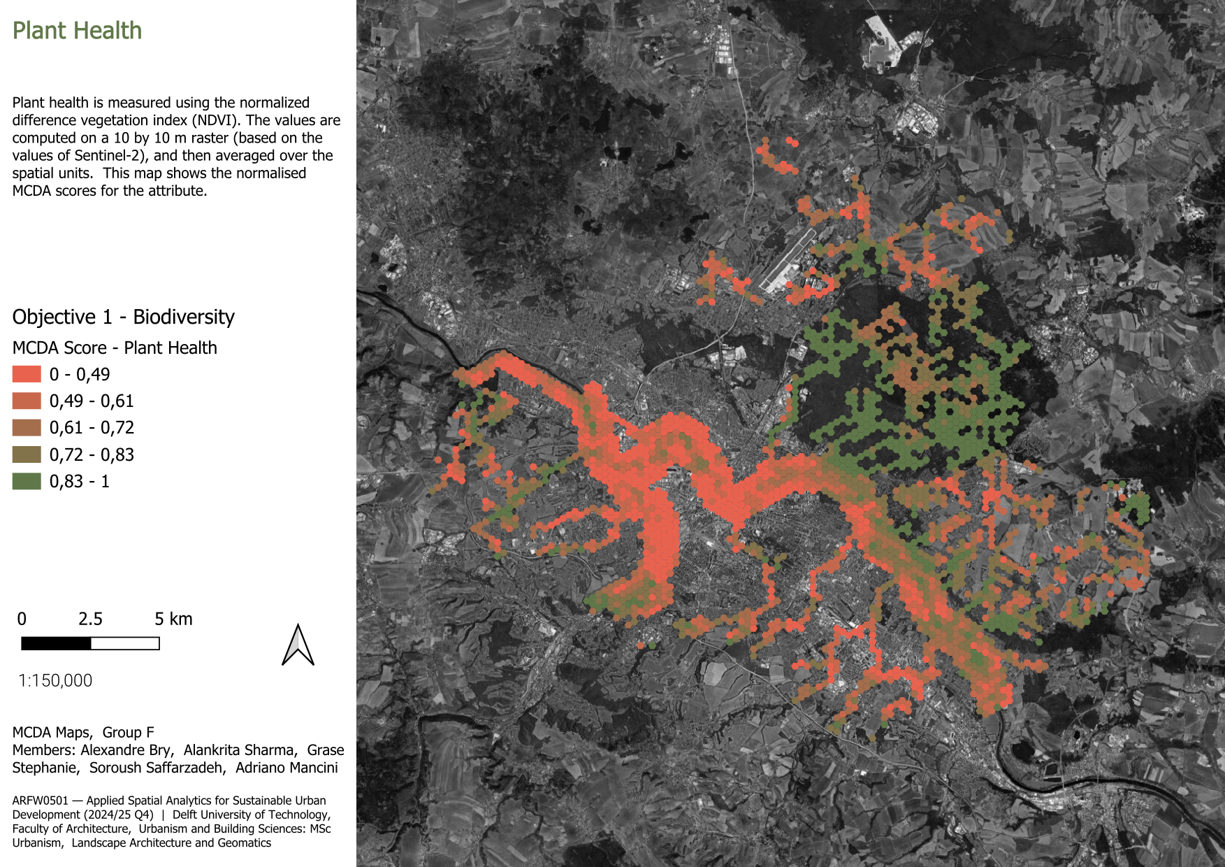
Plant health is measured using the normalised difference vegetation index (NDVI), computed as an average of the values in June, July and August (when the vegetation is facing the highest stress) over the five last available years (2020-2024). The values are computed on a 10 by 10 m raster (based on the values of Sentinel-2), and then averaged over the spatial units. Higher values correspond to healthier vegetation.
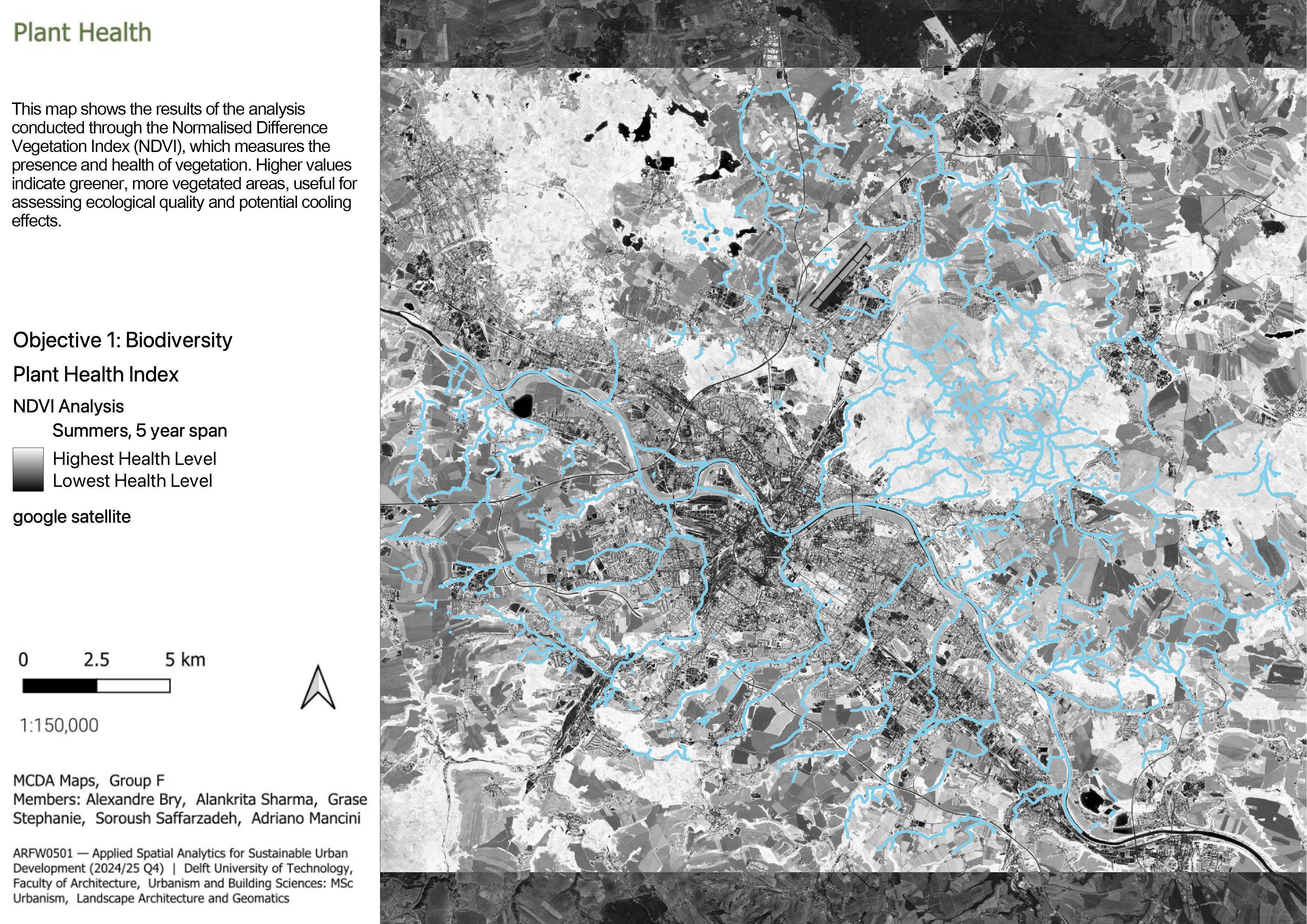
The code that was used to compute the NDVI on the whole area is available in Section 1 in the appendix.
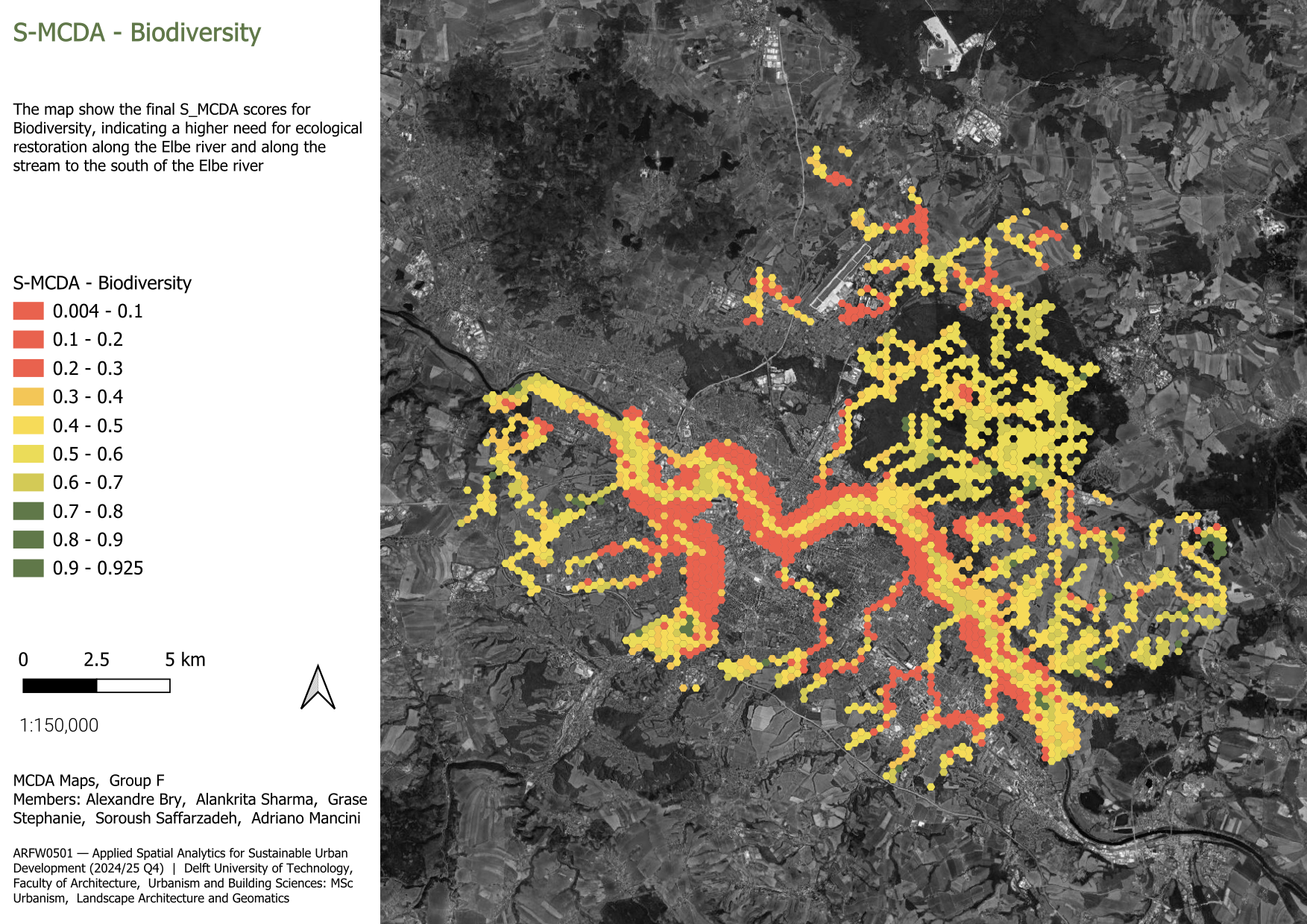
3.1.1.4 Conclusion - Biodiversity
In conclusion, It can be noted that there is a higher need for ecological restoration along the Elbe river and along the stream to the south of the Elbe river.
3.1.2 Climate Adaptation
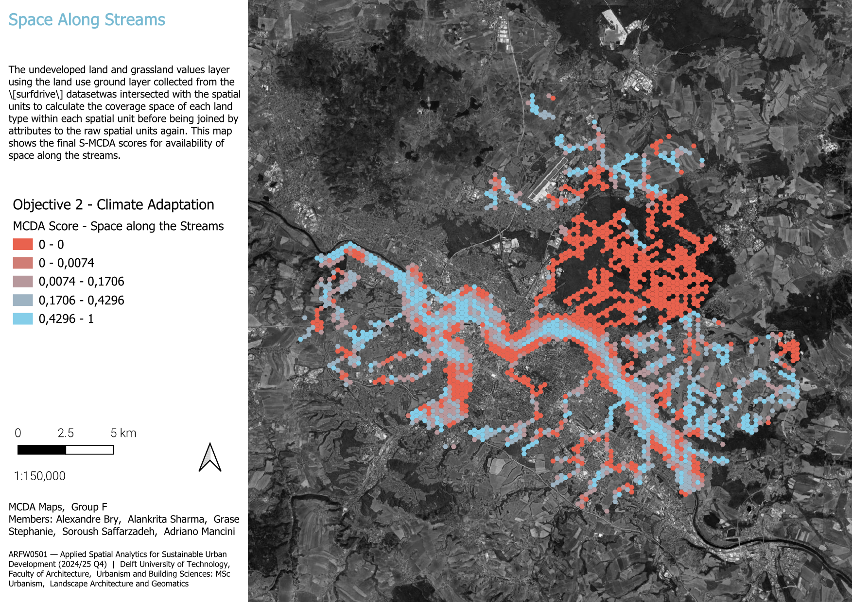
3.1.2.1 Available space near streams
The necessity of available open space along the streams and the water body will be a potential opportunity for design interventions to prevent, or at least reduce, the flood risk along the streams’ banks. This can be achieved by calculating the available open space areas in the close proximity of the streams and rivers of Dresden.
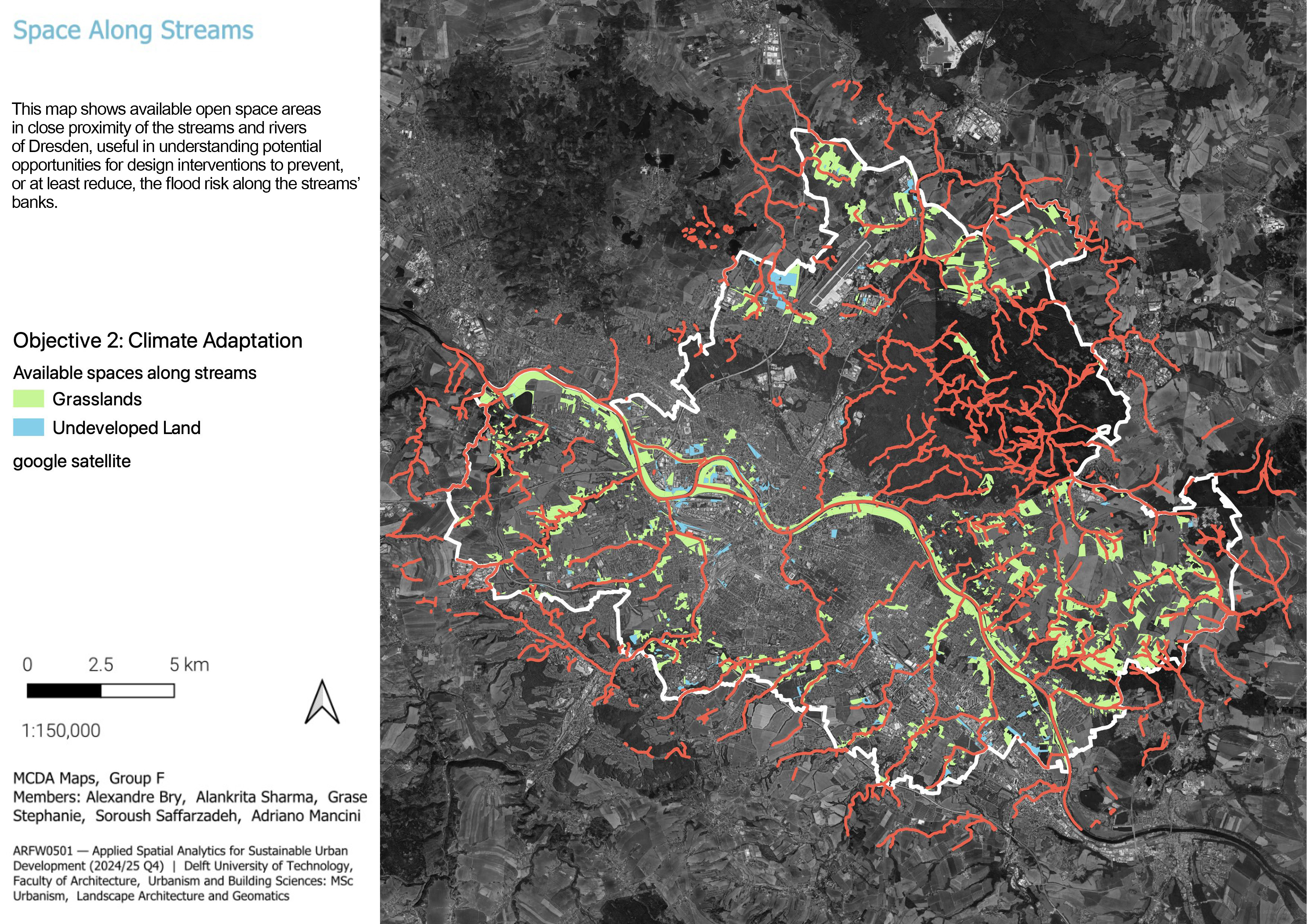
This was assessed by using the land use ground layer collected from the [surfdrive] dataset and filtered based on the undeveloped land and grassland values. After that, the layer was intersected with the spatial units to calculate the coverage space of each land type within each spatial unit before being joined by attributes to the raw spatial units again.
By joining the intersected layer to spatial units based on their join attributes, the available space within each spatial unit is already available. In order to normalize the values, the area values were all divided by the highest area number, and the new results were distributed between zero, as the lowest coverage or available area, and one, as the highest coverage and available area.
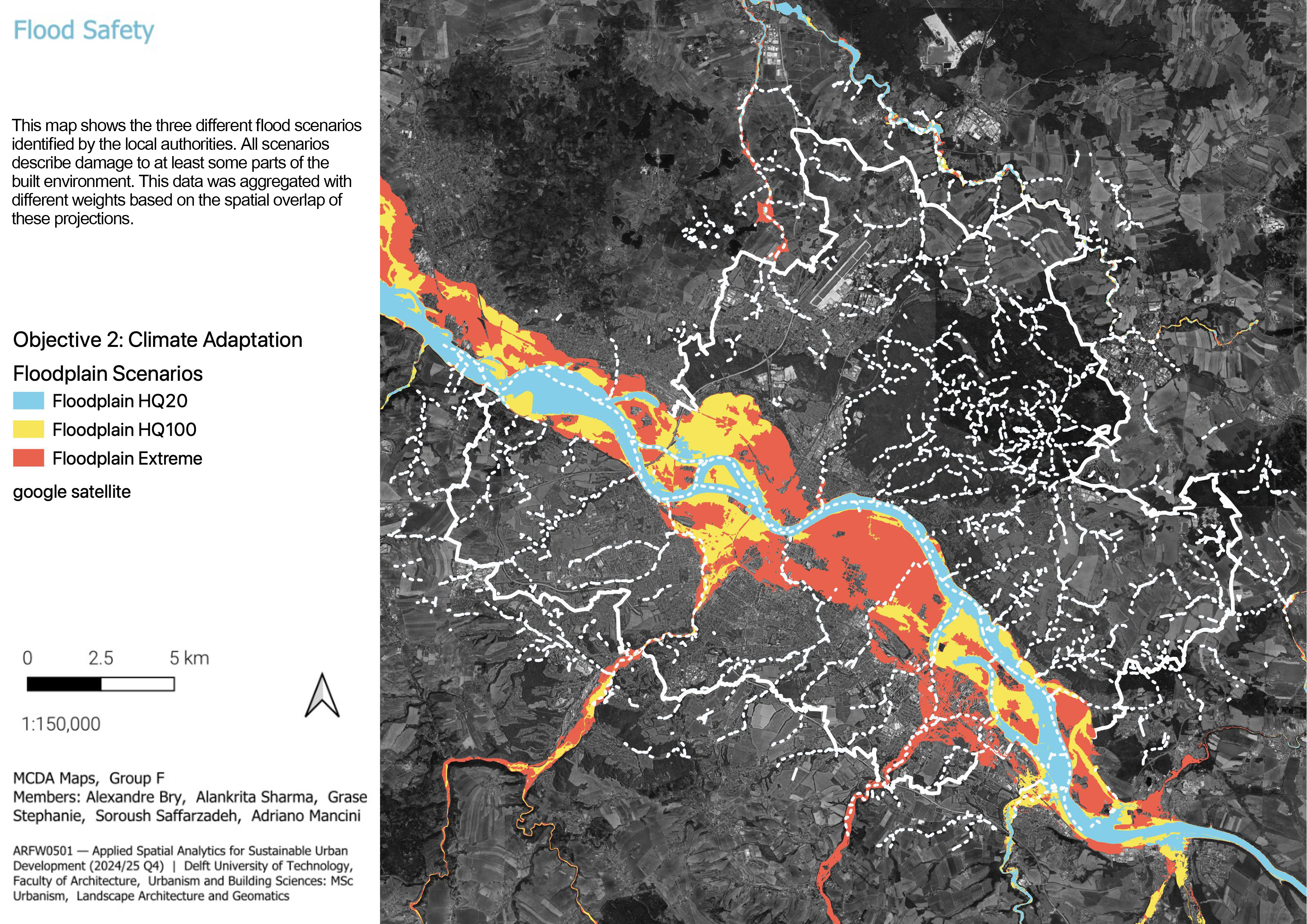
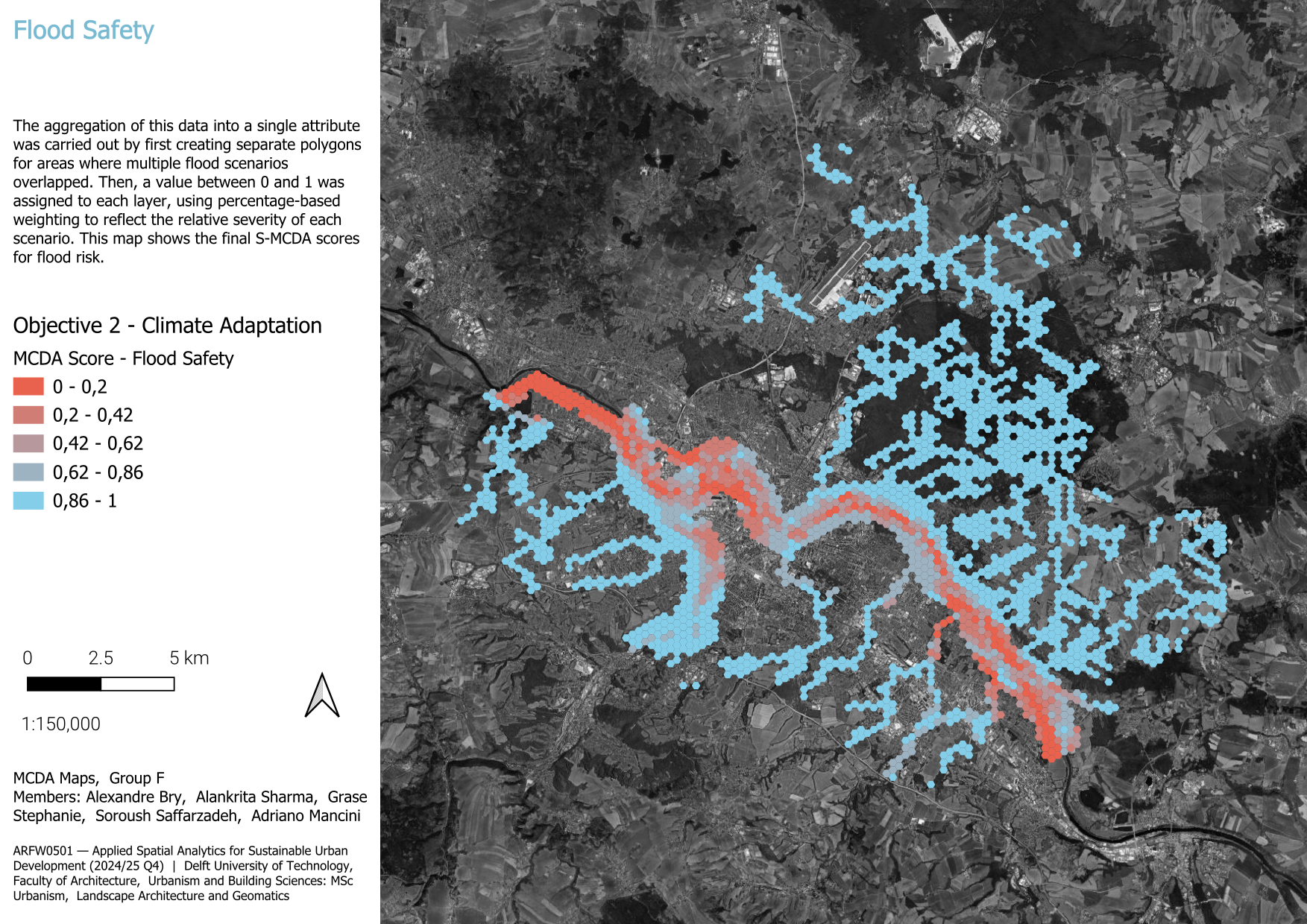
3.1.2.2 Flood Safety Index
The flood hazard data used in our analysis originate from official Saxon authorities and were developed as part of a study commissioned by the Civil Engineering Office in 2020, following new regional legislation on flood protection. A rainfall-runoff model was used to simulate three flood scenarios: events expected every 20 years (HQ20), 100 years (HQ100), and an additional extreme scenario. These simulations resulted in spatial layers indicating areas affected under each condition.
We created a Flood Safety Index on a scale from 0 to 1 (0 = highest exposure, 1 = safest). The process began by overlaying the three flood hazard scenarios:
- HQ20 (frequent flood events)
- HQ100 (centennial flood events)
- Extreme events (likely representing HQ200 or catastrophic scenarios)
Each flood layer was treated as a binary indicator of hazard presence. We assigned simple weights based on perceived severity:
- Extreme events → 0
- HQ100 → 0.33
- HQ20 → 0.67
- Areas outside all flood zones → 1
To compute values per spatial unit, we overlaid the flood polygons with our analysis grid and calculated the area-weighted average of hazard severity values – accounting for the portion of each polygon within a unit. These averages were then normalized to a 0–1 scale.
While this method does not reflect depth, speed, or return probabilities, it enables basic spatial prioritization. We acknowledge its limitations but consider it useful for exploratory and comparative planning purposes.
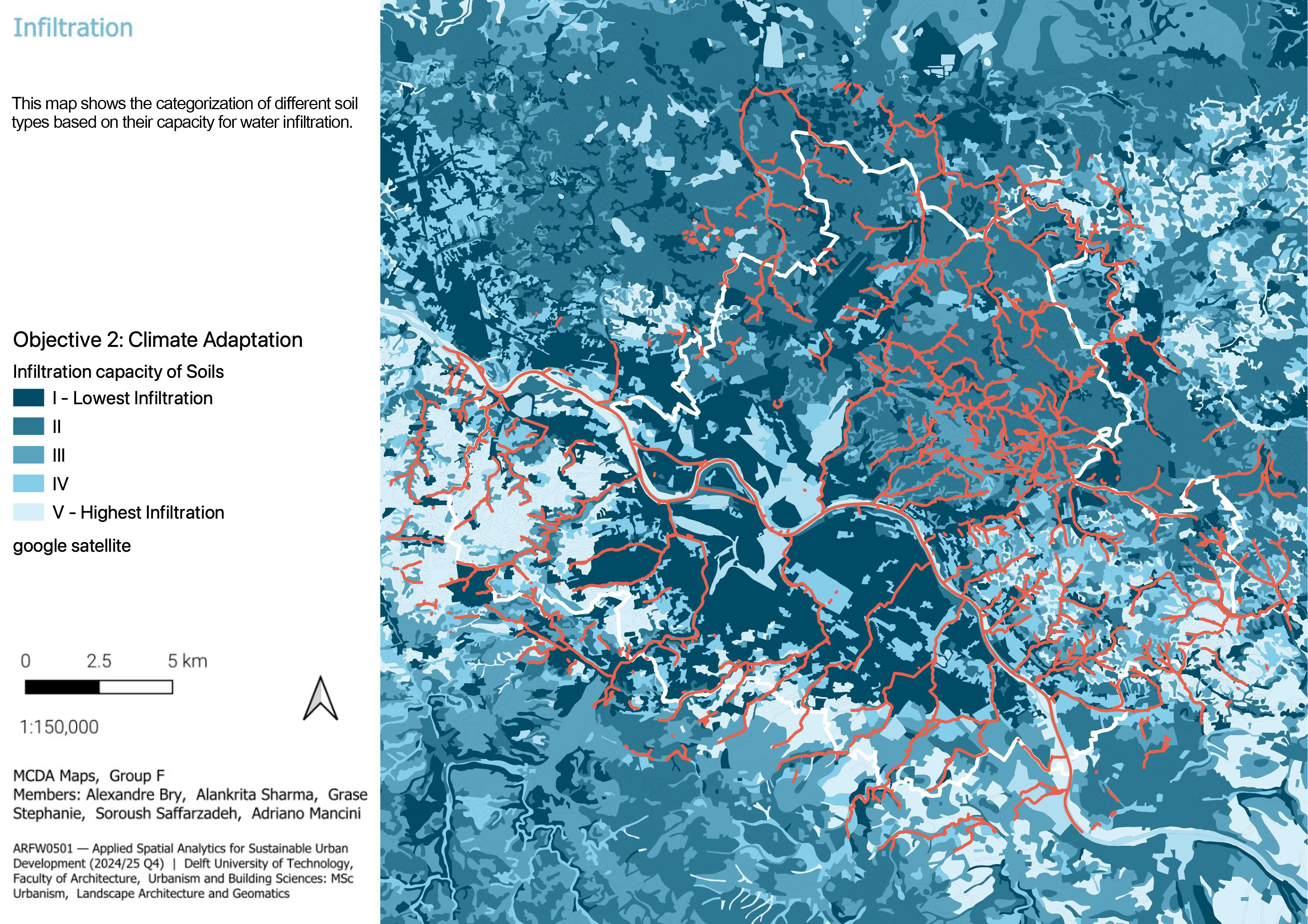
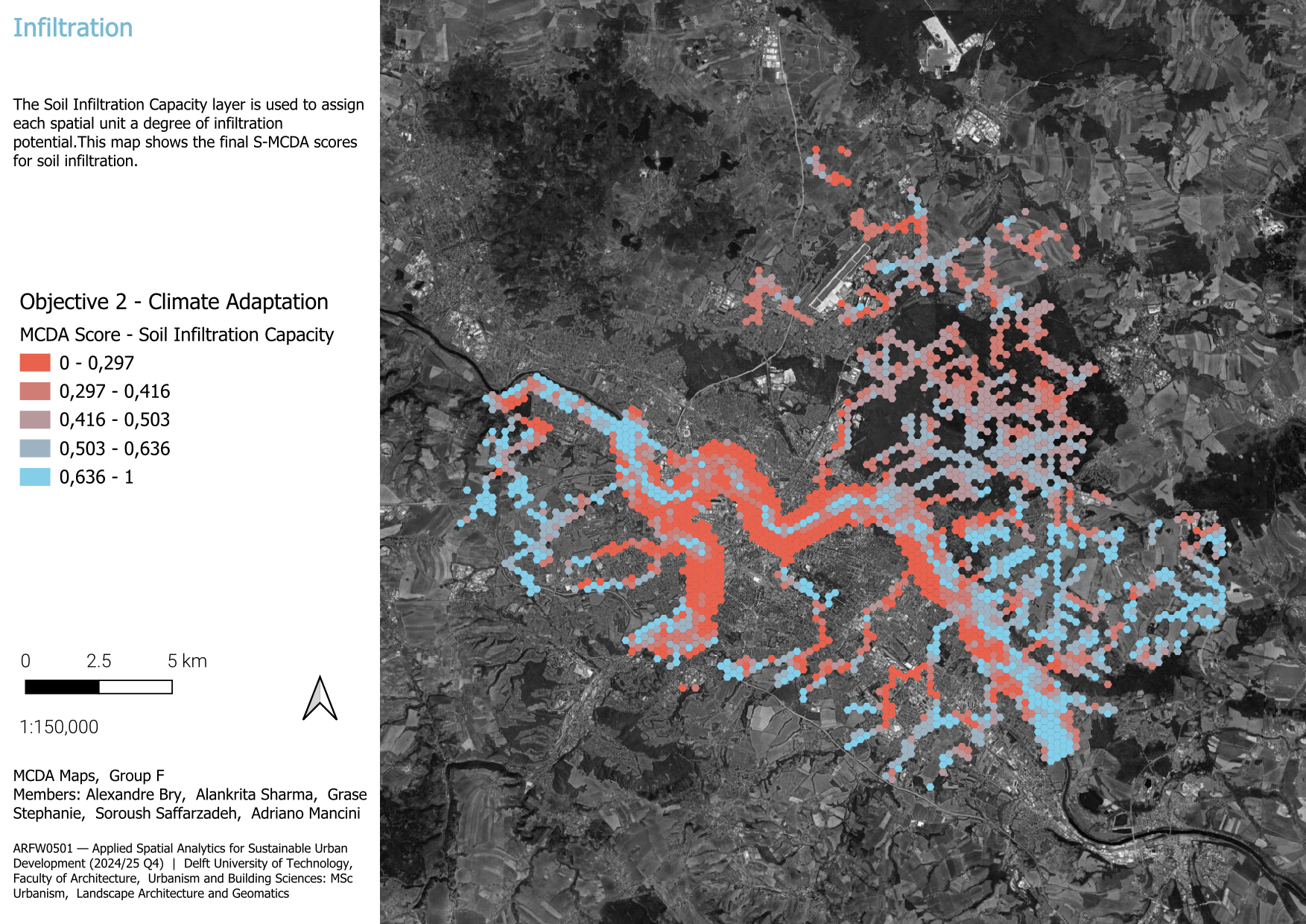
3.1.2.3 Soil infiltration capacity
To operationalize the infiltration capacity data, we accessed the Wasserspeichervermögen des Bodens WFS layer, which contains classified polygons showing estimated infiltration potential across Saxony. The classes were interpreted as follows:
- Very low infiltration → 0
- Low → 0.25
- Medium → 0.5
- High → 0.75
- Very high → 1
We intersected this dataset with our spatial units and computed the area-weighted average of the infiltration values per unit – accounting for the share of each infiltration class polygon within a spatial unit. This yielded a single score per unit, which we then normalized to a 0–1 scale for comparability.
The resulting Infiltration Index offers a simplified but spatially meaningful way to assess soil permeability and its contribution to local water resilience.
3.1.2.4 Shade
By knowing the shade coverage of open spaces across the stream area networks, the potential areas for heat resilience can be spotted. Also, the open spaces that have the highest exposure to the heat waves can be recognized through the ground shadow analysis, especially during the peak time of warm periods in the area.
The DSM and DTM raster layers were needed to run the shadow analysis based on the Section 2 and vegetation heights. The raster layer was clipped out based on the dissolved layer of spatial units to limit the area of analysis. The buildings layer was also masked out from the DSM layer and patched with it again to represent the updated building heights. After that, the aspect and edge heights were calculated using the UMEP plugin to process the preliminary data for the shadow analysis. The shadow analysis is done at 15:00 within the peak time of warm period in the area which is July 15th, 2024 in Dresden.
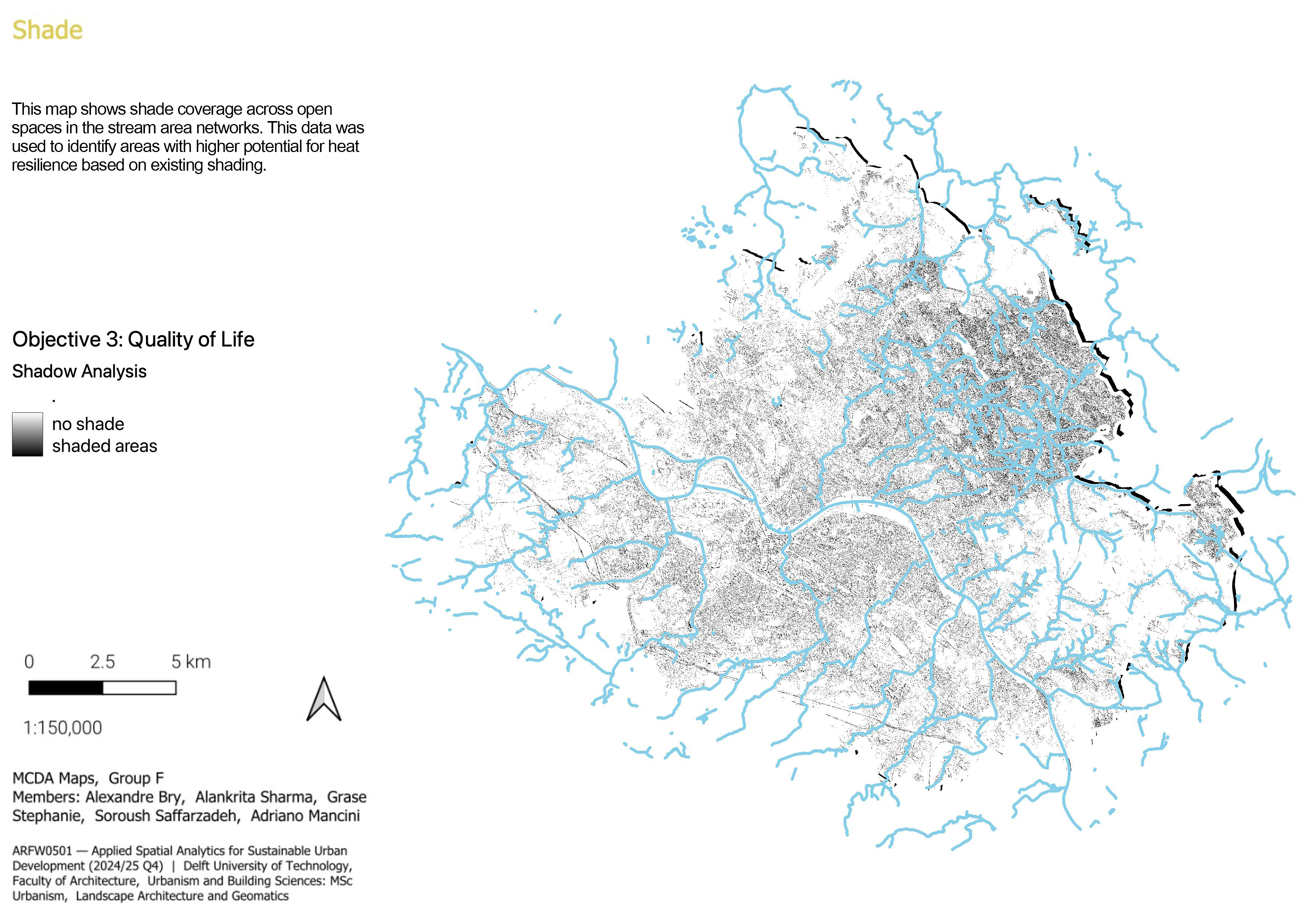
The output layer with which was a raster layer, was then aggregated to the spatial units using the Zonal Statistics tool to translate the shading values to the polygon spatial units. The output values were the counted illuminated values divided by each pixel contained within each spatial unit. After that, to define the lowest value as no shadow, the attributes were inverted by this equation:
\[ \text{Proportion\_Shaded} = 1 - \left(\frac{\text{Count\_Illuminated}}{\text{Count\_Pixels}}\right) \]
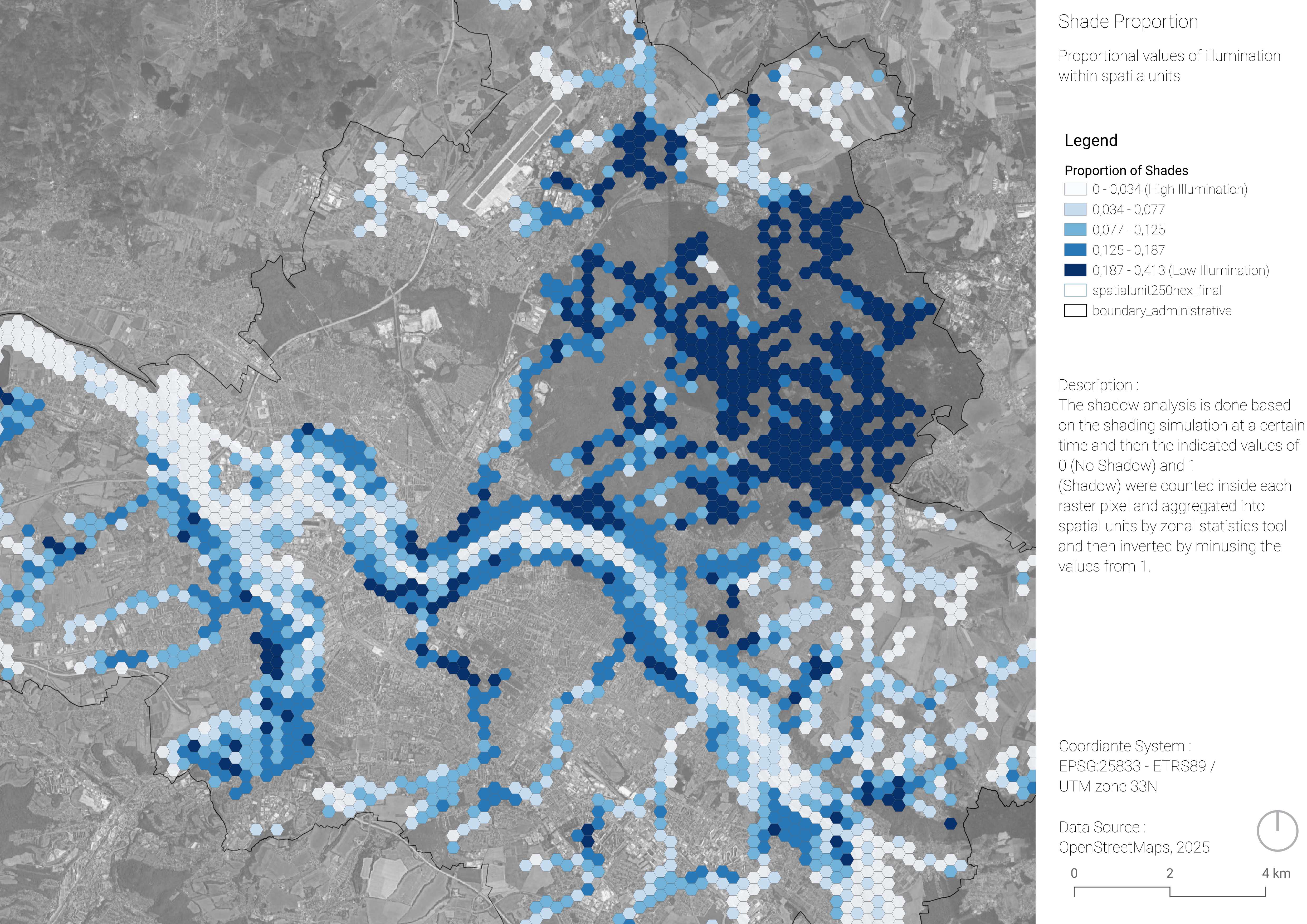
To normalize the proportioned values, the attribute values were divided by the attribute with the highest value (i.e. 0.4133) since the minimum values is zero and is a meaningful one, then the normalization could be done only by dividing all values by the maximum value:
\[ \text{Normalised\_Value} = \left(\frac{\text{Proportion\_Shaded}}{0.4133}\right) \]
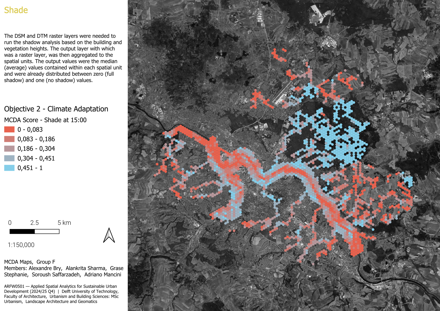
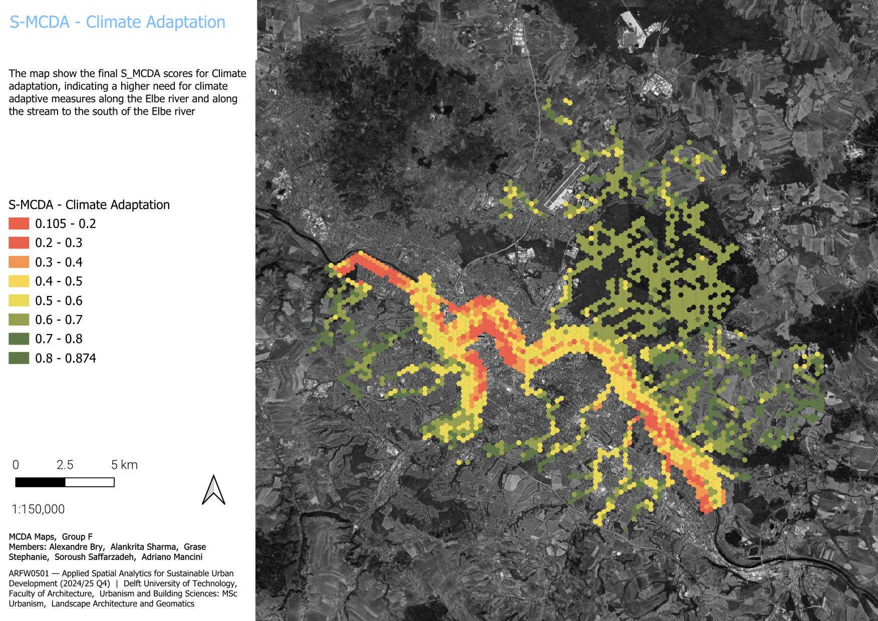
3.1.2.5 Conclusion - Climate Adaptation
In conclusion, It can be noted that there is a higher need for climate adaptive measures along the Elbe river and along the stream to the south of the Elbe river.
3.1.3 Quality of Life
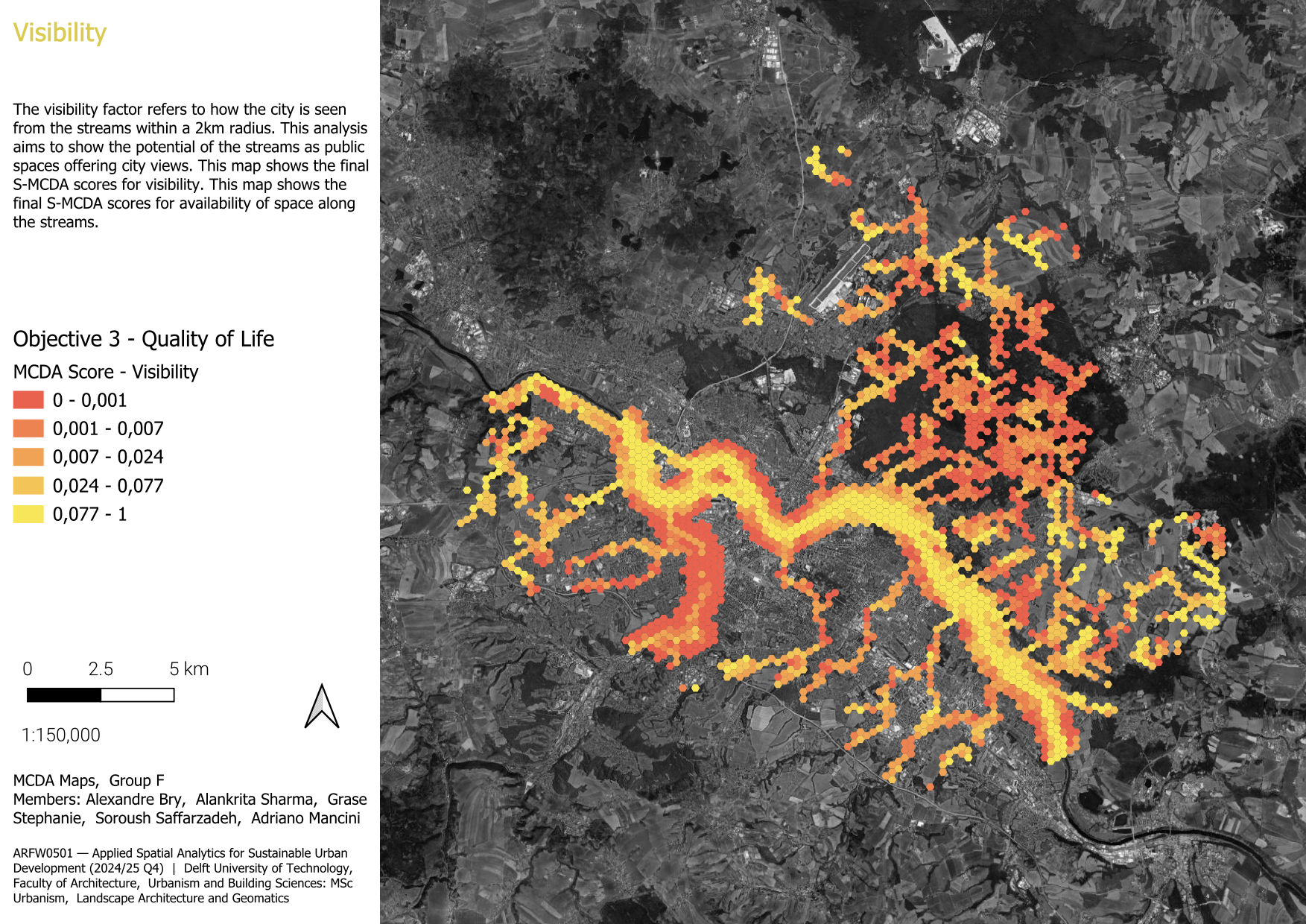
3.1.3.1 Visibility
The visibility factor refers to how the city is seen from the streams within a 2km radius. This analysis aims to show the potential of the streams as public spaces offering city views. When many parts of the city are visible from the stream corridors, it can show the contribute to their attractiveness. These are the steps we followed:
- Interpolated points from the streams’ center lines at 500 m intervals, with the assumption these points can represent the overall visibility from the streams.
- Created viewpoints using the interpolated points as the observer location with a height of 1.6 m (eye level). In this step, we used DSM model as it considers not only elevation but also other features such as buildings and trees that might block the view.
- Limited and set the radius of the analysis to 2km, as this is considered an ideal distance. The physical aspects of objects remain visually recognizable within this range.
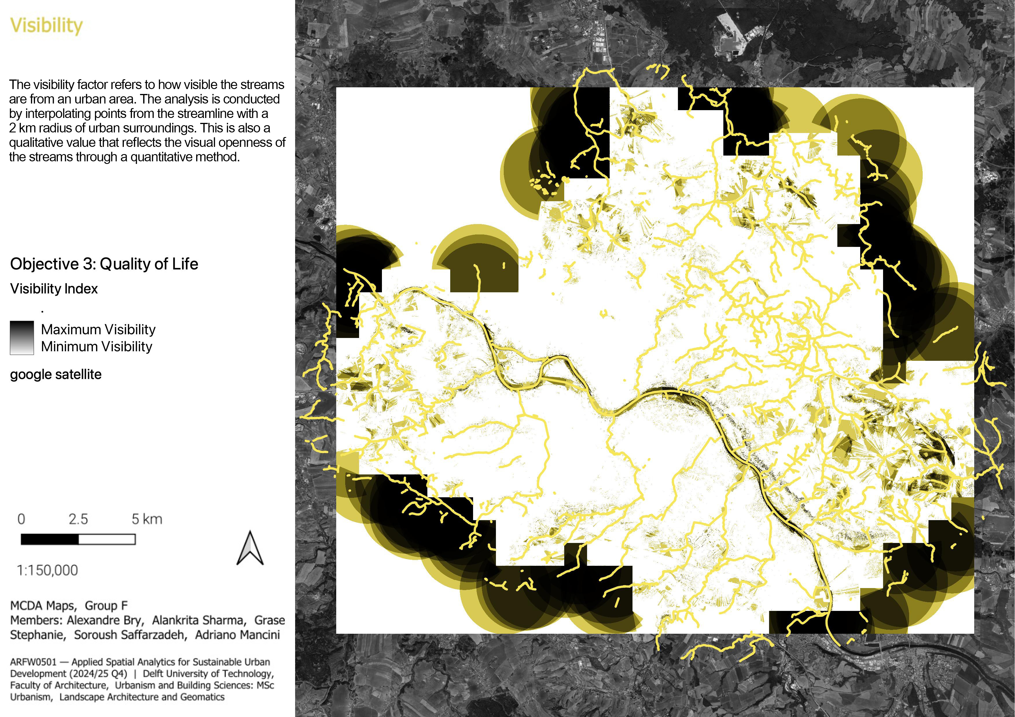
The output layer, in raster format (.tiff), was aggregated into spatial units using zonal statistics tool. Then, the values were normalised to a 0–1 range by dividing each value by the maximum value, where higher values indicate greater visibility from the streams.
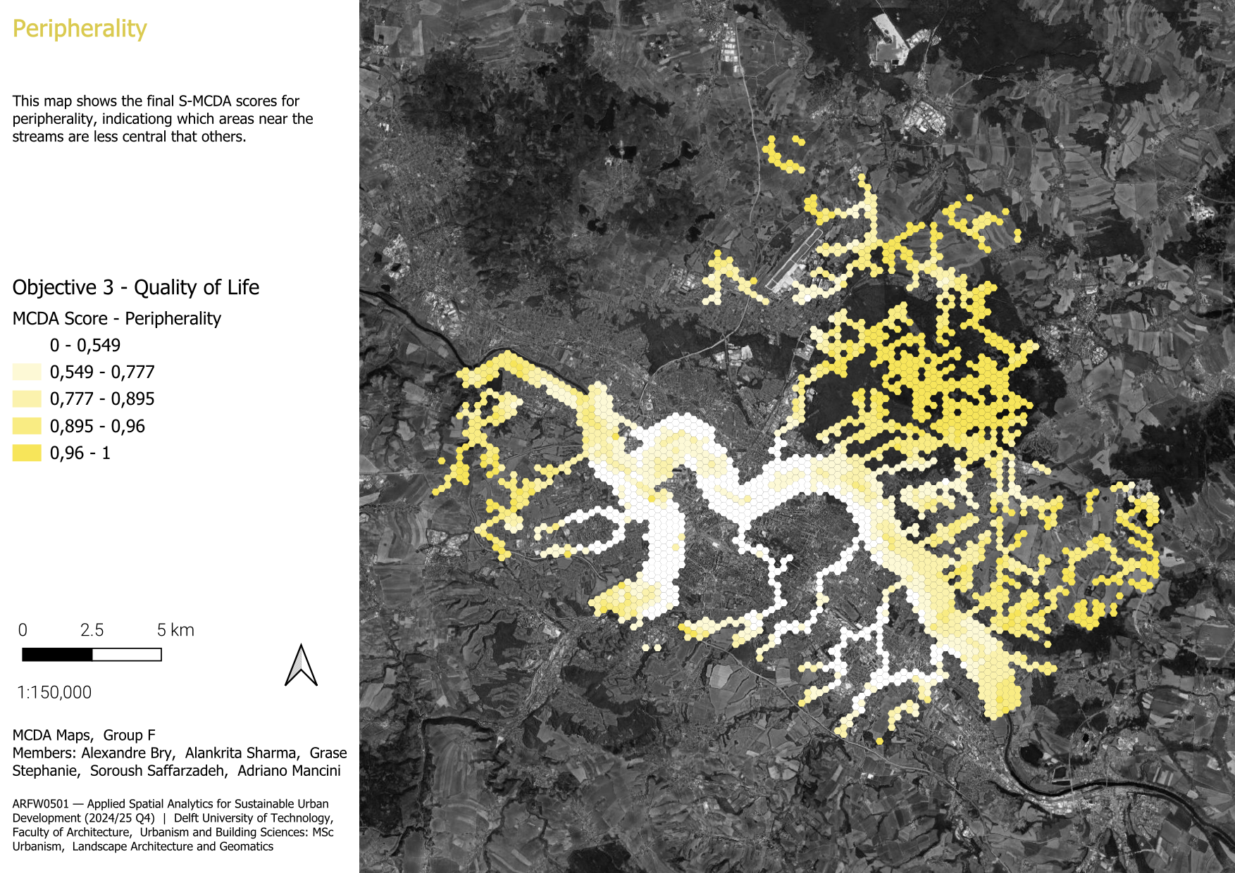
3.1.3.2 Peripherality
The idea behind the peripherality is that for the quality of life, spatial units that are closer to places where inhabitants live are more valuable and more important than those that are harder to reach. Therefore, we wanted to study how many people leave close to each spatial unit, and are therefore accessible by feet. To do so, we settled on a threshold of 1km for the maximum distance that makes a spatial unit accessible, and we used the following steps to compute the accessibility:
- Extract the center point of each spatial unit. These will serve as destination points for the spatial units.
- Sample points on a 200m×200m grid and only keep those in a 1km buffer around the spatial units. These will serve as start points representing where people live. Assign to each of these points a population density based on the density grid 1000m×1000m of Germany in the year 2020.
- Compute the paths between all pairs of start and destination points. We used the roads from OpenStreetMap. Using this layer required to clean up some isolated roads, because some starting points or spatial units centered would be attached to parts of the network that were not connected to the rest, and therefore it was not possible to find paths. To identify them, we run the path computation from all points to one point, and then manually removed parts of the network that were isolated and preventing the algorithm from finding paths.
- Keep only the paths that are shorter than 1km, representing convenient accessibility by feet.
- Compute the accessibility of each spatial unit \(\text{su}\) as: \[\text{accessibility}(su) = \sum\limits_{sp \;\in\; \text{Starting points}} \text{population}(sp) \times (2000 - \text{distance}(su,sp))\] The reason for using 2000m as a basis is so that a 0m distance has two times more value than a 1000m distance (the maximum we kept).
- Normalise the accessibility between 0 and 1 and compute the peripherality as \(1 - \text{accessibility}_\text{normalised}\).
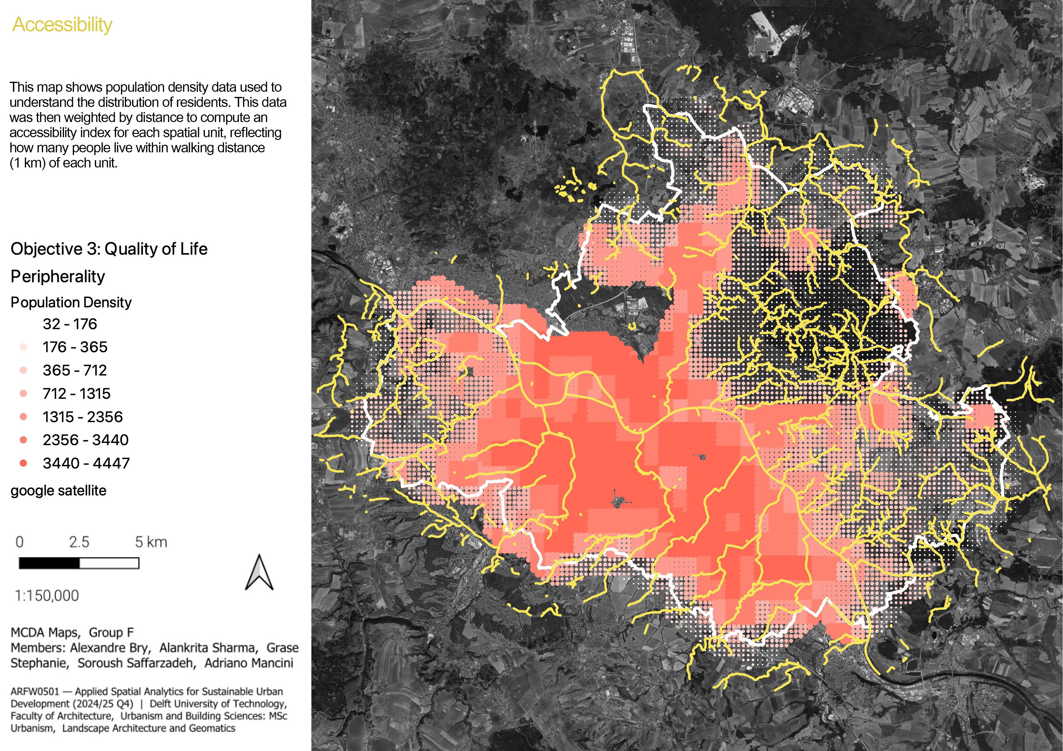
The final value is not really interpretable, as it is a population density multiplied by a distance, but it gives us a good indication of spatial units that are the most accessible.
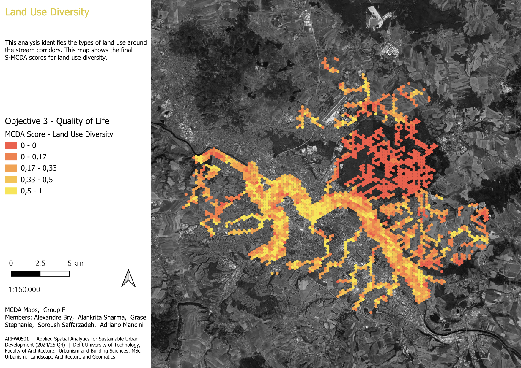
3.1.3.3 Land use variety
This analysis identifies the types of land use around the stream corridors. The more variety of uses enhances the connectivity of streams with the current urban fabric. When areas around the streams include a mix of public spaces, amenities, residential areas, and commercial or institutional functions, the streams become more integrated into everyday urban life. For this purpose, the land use data was simplified into 10 main categories.
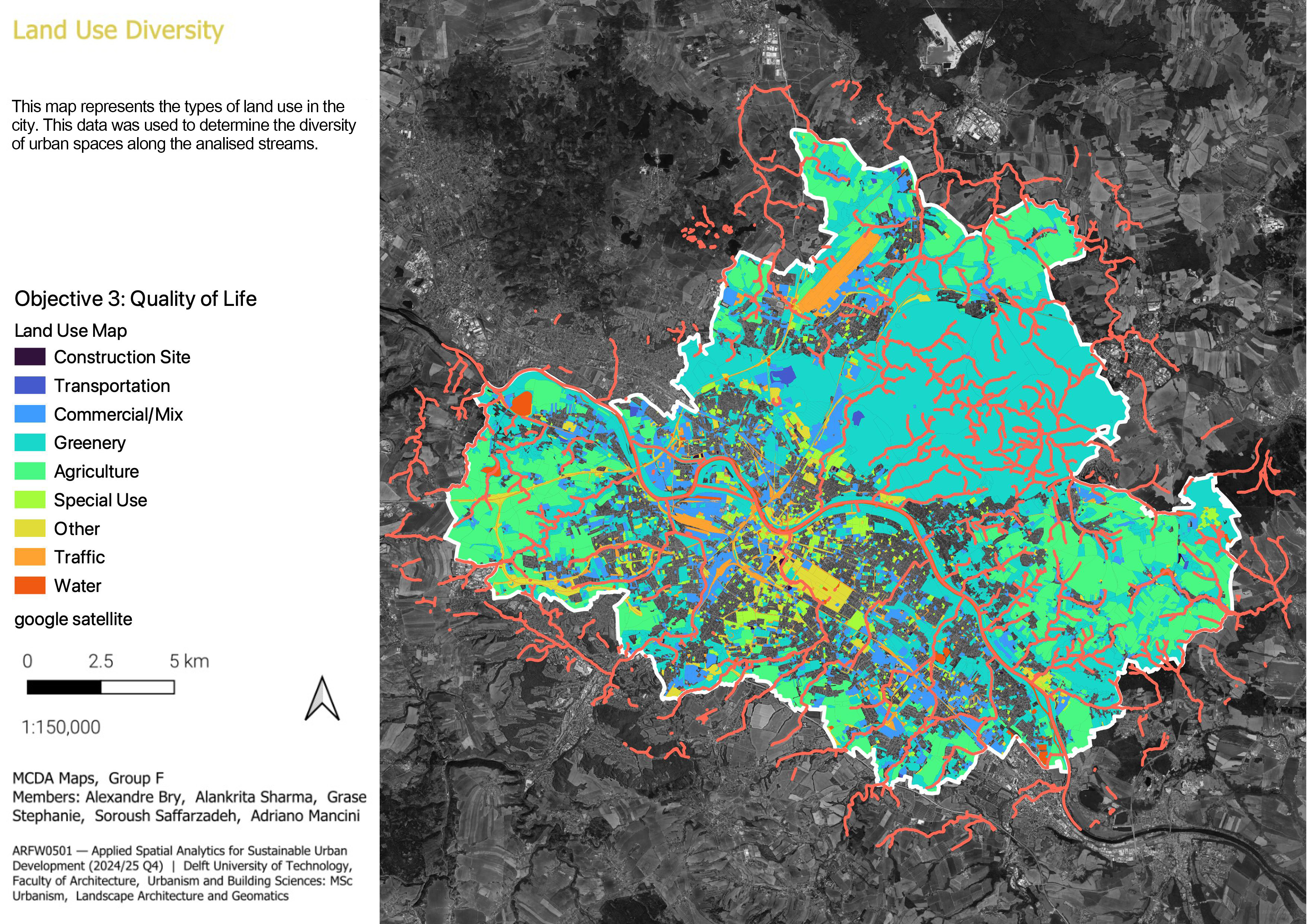
Using this data, the diversity of land use within each spatial unit was measured, and the results were expressed through a value assigned to each unit. Then, the values were normalised within the range between 0-1 by dividing each value with the maximum value. Areas with high values indicate greater diversity in land use.
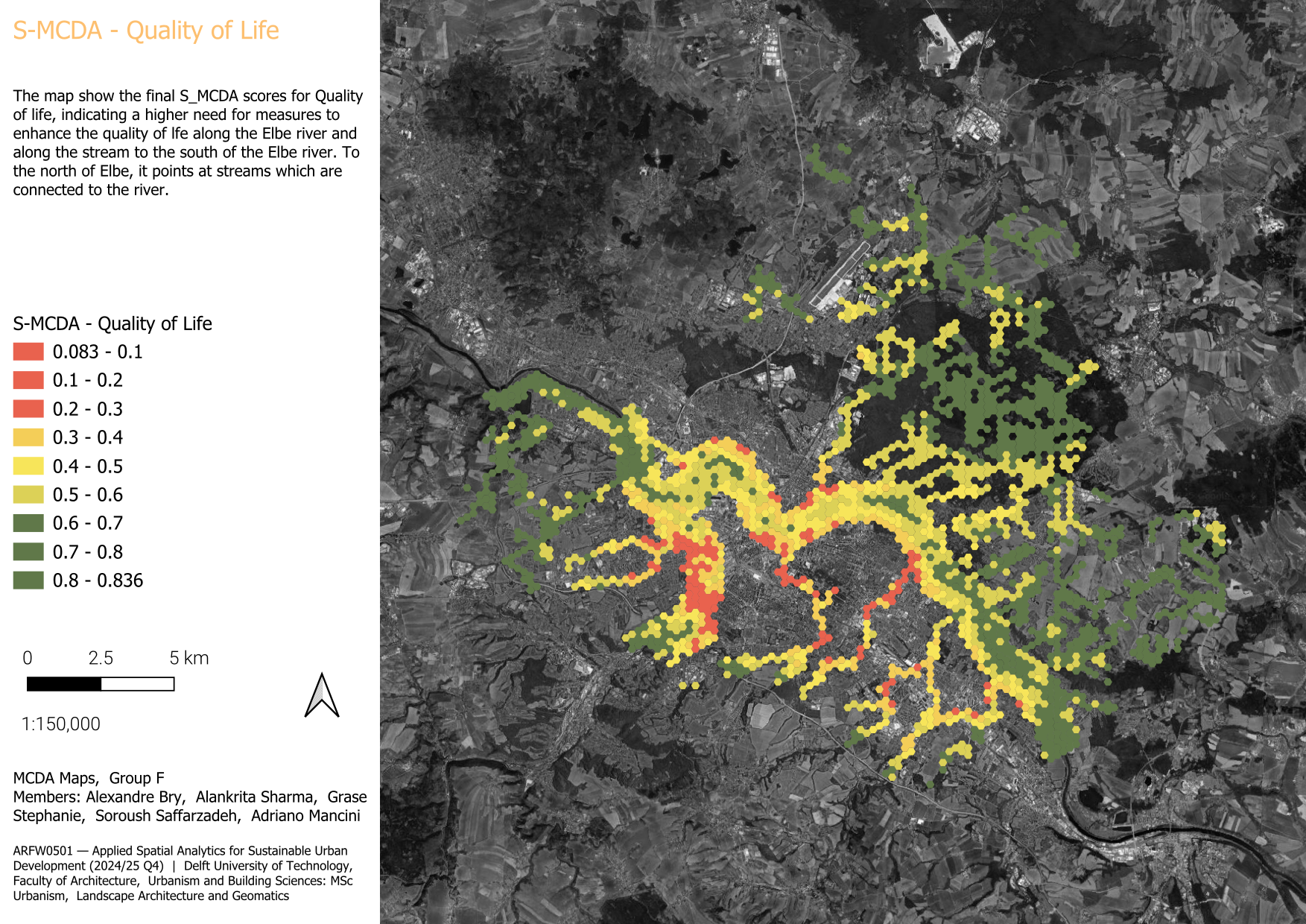
3.1.3.4 Conclusion - Quality of Life
In conclusion, the results indicate a higher need for measures to enhance the quality of life along the Elbe river and along the streams to the south of Elbe river. To the north of river, it points to the streams which are connected to river.
3.2 Weighting of the Attributes
Once each attribute has produced a normalised value for each spatial unit, all the attributes need to be aggregated into one final value. Since all of them do not participate equally to the goals we mentioned earlier, we tried to weight them according to their relative importance in achieving our goals. These weights could then be used to compute a weighted average that is easier to use thanks to reducing the problem to one dimension instead of several dimensions.
To compute the weights, we made individual Saaty matrices for the attributes of each of the three objectives. Saaty matrices are square matrices that allow us to deduce weights from pairwise comparisons of the attributes (Saaty 1987). In our case, we used the eigenvector method to calculate the weights. The matrices and weights are shown in Table 3.1 below.
Then, we divided them by 3 to assign the same weight to the three attributes, and got a final set of weights that summed to 1. We chose this method because it allowed us to assign more weights to the most reliable and pertinent attributes, while maintaining the balance between the three main objectives.
| Soil quality | Plant health | Green-blue connectivity | |
|---|---|---|---|
| Soil quality | 1 | 3 | 4 |
| Plant health | 1/3 | 1 | 2 |
| Green-blue connectivity | 1/4 | 1/2 | 1 |
| Weights | 0.625 | 0.238 | 0.136 |
| Available space near streams | Anticipated flood risk | Soil infiltration capacity | Shade | |
|---|---|---|---|---|
| Available space near streams | 1 | 1/2 | 1/3 | 2 |
| Anticipated flood risk | 2 | 1 | 3 | 4 |
| Soil infiltration capacity | 3 | 1/3 | 1 | 3 |
| Shade | 1/2 | 1/4 | 1/3 | 1 |
| Weights | 0.158 | 0.471 | 0.280 | 0.090 |
| Visibility | Peripherality | Land use variety | |
|---|---|---|---|
| Visibility | 1 | 1/4 | 1/2 |
| Peripherality | 4 | 1 | 3 |
| Land use variety | 2 | 1/3 | 1 |
| Weights | 0.136 | 0.625 | 0.238 |
These weights were computed with respective consistency ratios of 0.016, 0.081, and 0.016 for Biodiversity, Climate Adaptation, and Quality of Life. These values are below the threshold of 0.1 prescribed by Saaty (1987), which indicates that the pairwise comparisons were consistent enough to be used in the analysis.
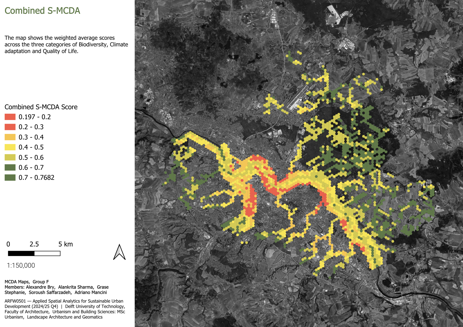
3.3 Results of the Analysis
The average value of all three categories represents the considerable environmental quality caused by the streams across the city of Dresden. The overall higher values are concentrated in the southern bank of Elbe river and some clusters in the far east in the outskirts of the city. Moreover, there are smaller spots along the river bank zones that lack sufficient values. Although the urban streams represent a reasonable environmental quality around their buffers, the Elbe river holds some areas of lower quality that draws the attention for intervention. The average value of all three categories represents the considerable environmental quality caused by the streams across the city of Dresden. The overall higher values are concentrated in the southern bank of Elbe river and some clusters in the far east in the outskirts of the city. Moreover, there are smaller spots along the river bank zones that lack sufficient values. Although the urban streams represent a reasonable environmental quality around their buffers, the Elbe river holds some areas of lower quality that draws the attention for intervention.