Appendix

NDVI Computation

The code chunk that we used to compute the NDVI from Google Earth Engine is shown below. It actually computes the NDVI as well as two other indices (NDREI and NDWI) that we ended up not using for our analysis. You can easily compute other indices with the library that is used, by changing the variable called indices. Furthermore, it computes an average on the last five years, roughly for each season, and exports the data to Google Earth Engine. You might have to change the output path to adapt it to your situation in the call to the function Export.image.toDrive. Finally, this algorithm requires an extent (a vector layer) as an input that defines the area of interest. This can be changed in the variable called extent.

var extent = ee.FeatureCollection("projects/arfw0501/assets/Spatial_units_extent");

var spectral = require("users/dmlmont/spectral:spectral");

// Indices to compute
var indices = ["NDVI", "NDREI", "NDWI"];

// Get the bounding box of the shapefile and buffer it
var bbox = extent.geometry().bounds();
var bbox_utm = bbox.transform('EPSG:25833', 0.1);
var bbox_wgs84_buffered = bbox_utm.transform('EPSG:4326', 0.1).buffer(3000);

// Center the map
Map.centerObject(bbox_wgs84_buffered, 12);

// Define seasons and their date patterns
var seasons = [
  {name: 'Winter', start: '-12-01', end: '-02-28', lastStartYear: 2024},
  {name: 'Spring', start: '-03-01', end: '-05-31', lastStartYear: 2024},
  {name: 'Summer', start: '-06-01', end: '-08-31', lastStartYear: 2024},
  {name: 'Autumn', start: '-09-01', end: '-11-30', lastStartYear: 2024},
];

// Loop over each season
seasons.forEach(function(season) {
  // Create an object to store images for each index
  var indexImages = {};

  // Initialize empty lists per index
  indices.forEach(function(index) {
    indexImages[index] = [];
  });

  // Loop over the past 5 years
  for (var y = 0; y < 5; y++) {
    var year = season.lastStartYear - y;

    var startYear = year;
    var endYear = (season.name === 'Winter') ? year + 1 : year;

    var startDate = startYear + season.start;
    var endDate = endYear + season.end;

    // Load and filter Sentinel-2 imagery
    var collection = ee.ImageCollection('COPERNICUS/S2_SR_HARMONIZED')
      .filterBounds(bbox_wgs84_buffered)
      .filterDate(startDate, endDate)
      .filter(ee.Filter.lt('CLOUDY_PIXEL_PERCENTAGE', 10))
      .median();

    // Compute all requested indices
    var parameters = {
      "S2": collection.select("B12"),
      "S1": collection.select("B11"),
      "N2": collection.select("B8A"),
      "N": collection.select("B8"),
      "RE3": collection.select("B7"),
      "RE2": collection.select("B6"),
      "RE1": collection.select("B5"),
      "R": collection.select("B4"),
      "G": collection.select("B3"),
      "B": collection.select("B2"),
      "L": 0.5
    };

    var computedIndices = spectral.computeIndex(collection, indices, parameters);
    computedIndices = computedIndices.clip(bbox_wgs84_buffered);

    // Add each computed index image to the relevant list
    indices.forEach(function(index) {
      indexImages[index].push(computedIndices.select(index));
    });
  }

  // Compute and display/export average per index for the season
  indices.forEach(function(index) {
    var meanImage = ee.ImageCollection(indexImages[index]).mean();
    
    // Display
    Map.addLayer(meanImage, {min: -1, max: 1, palette: ['red', 'white', 'green']},
      index + '_' + season.name + '_mean');

    // Export
    Export.image.toDrive({
      image: meanImage,
      description: index + '-' + season.name + '-mean_5yr',
      folder: 'EarthEngineExports',
      fileNamePrefix: index + '-' + season.name + '-mean_5yr',
      region: bbox_utm,
      scale: 10,
      crs: 'EPSG:25833',
      maxPixels: 1e13
    });
  });
});

Building Geometry

The process of fixing the geometries of the clipped building layer can be done through this text Since the building layer had several geometry errors, it went through some geometry validation and fixing processes (i.e. valid geometry, fix geometries, simplify and re-project). For a smoother experience, you can read through this process to fix your geometries:

1. “Use “Check Validity” Go to: Vector → Geometry Tools → Check Validity
2. Choose “GEOS” as the engine.
3. Review the reported issues — “valid” in QGIS may not be sufficient for overlay ops if robustness is compromised.
4. Fix Geometries (Again) Run: Vector → Geometry Tools → Fix Geometries

If already done, try exporting the layer as a new file (Right-click layer → Export → Save Features As…) to reset underlying geometry representations.

If you encountered errors for holes or self-intersections, Simplify or Snap Geometries Minor overlaps/gaps or very close vertices can trigger GEOS precision issues.

Try:

1. Vector → Geometry Tools → Snap geometries to layer
2. or Vector → Geometry Tools → Simplify Geometry
   Use “Invalid Geometry Handling” in Processing If using model/processing tools, go to the settings (Processing → Options) → “Invalid geometry handling” → set to “Ignore features with invalid geometries” (temporary workaround).
3. Use Buffer(0) as a Cleanup Trick. Use the expression:buffer($geometry, 0) in the Geometry by Expression tool.

It often resolves subtle robustness problems.

CRS Conflict

Your raster is in EPSG:25833, but you’re trying to extract it using a mask layer in EPSG:32633. These CRS look similar (both UTM zone 33N), but they’re not the same datum:

• EPSG:25833 → ETRS89 (used in Europe, based on stable tectonic plate)
• EPSG:32633 → WGS84 (global standard)

GEOS and GDAL can throw robustness errors if vector and raster CRS differ even slightly during masking.

Option 1: Reproject the Mask Layer to Match the Raster Right-click the mask layer → Export → Save Features As…

1. Set CRS to EPSG:25833
2. Use the new projected mask layer for extraction.
3. Raster → Extraction → Clip Raster by Mask Layer
4. Use this EPSG:25833 version of the mask

Option 2: Reproject the Raster Instead If the mask needs to stay in 32633, reproject the raster:

1. Raster → Projections → Warp (Reproject)
2. Target CRS: EPSG:32633

Resampling: Nearest neighbour (for categorical) or Bilinear (for continuous)

1. Save as new GeoTIFF
2. Then run the extract using the reprojected raster.

Always ensure both raster and mask have the exact same CRS (code and datum), not just similar projection zones. Otherwise, operations like masking can fail due to subtle misalignments or geometry issues.

Nested Holes Error

Furthermore, if you received such error:

Warning 1: Holes are nested at or near point 403128.48007987819 5659925.564998446ERROR 1: Cutline polygon is invalid. This means your cutline (mask) layer dissolved_fixed_reprojected.shp has self-intersecting or nested holes. GDAL (gdalwarp) cannot use this geometry until it is fully valid and simplified.

Final Fix — Repair Deep Geometry Issues Do the following in exact order:

Explode MultiParts Vector → Geometry Tools → Multipart to Singleparts → Run it on dissolved_fixed_reprojected.shp → Save result as e.g. dissolved_singleparts.shp

1. Use “Buffer(0)” Trick Open Processing Toolbox
2. Use Geometry by Expression on the singlepart layer
3. Expression:buffer($geometry, 0)
4. Save as: dissolved_cleaned_buffer0.shp

This rewrites the geometry and usually removes nested holes and invalid rings.

Final Geometry Check:

1. Run Check Validity tool on dissolved_cleaned_buffer0.shp
2. GEOS engine

All features must be valid

Reproject This Layer (if needed) If your raster is in EPSG:25833, make sure this cleaned mask is also in EPSG:25833.

Few Invalid Geometries

If you found a few invalid geometries after running Check Validity, do this:

Fix Them Properly (Step-by-Step)

1. Isolate Invalid Features Open the Check Validity output layer (or attribute table):
2. Filter by “valid” = ‘0’
3. Select all invalid features
4. Fix Individually or in Batch Use either:

A. Manual Fix:

1. Enable editing
2. Use vertex tool to correct overlapping rings, holes, etc. Useful for <10 features

B. Automated Fix:

1. Select invalid features
2. Run: Vector → Geometry Tools → Fix Geometries
3. Only apply to selected features
4. Save as fixed_invalids.shp
5. Replace Invalids in Main Layer Use “Merge Vector Layers”: Input: your original cleaned valid layer + fixed_invalids.shp
6. Output: final_cleaned_mask.shp

If you faced such error:

Warning 1: Too few points in geometry component at or near point 7143.291…ERROR 1: Cutline polygon is invalid.

It means you have “degenerate geometries” in your “valid” features — like a polygon made from just 1 or 2 vertices, which isn’t a valid polygon for GDAL.

Solution: Remove Features with Too Few Vertices

1. Open the attribute table of valid_only_mask_readyformask.shp
2. Use this filter in the expression dialog:num_points(\$geometry) \>= 4
3. Export the selected features:
4. Right-click → Export → Save Selected Features As…
5. Name it valid_clean_mask.shp
6. Optional: Run Buffer(0) Again Just to be sure:
7. Geometry by Expression Use: buffer($geometry, 0)
8. Save result as final_cutline_mask.shp
9. Retry Clipping Now use final_cutline_mask.shp as your cutline.

This should fully eliminate:

• Nested holes
• Invalid rings
• Too-few-points geometries

Self-intersection, Small rings or Overlapping vertices error

If you faced this error:

Warning 1: Self-intersection at or near point … ERROR 1: Cutline polygon is invalid.

means even after filtering and buffering, some geometries still have self-intersections, often caused by very small rings or overlapping vertices introduced during buffering or fixing.

Final Clean Repair: Force Rebuild of Valid Topology Do this:

1. Use Delete Holes Vector → Geometry Tools → Delete holes
2. Input: final_cutline_mask_buffered.shp
3. Keep minimum area very small (e.g. 0.0001)
4. Save as final_noholes.shp
5. Simplify + Buffer(0) Combo Now:
6. Run Simplify Geometry:
   1. Tolerance: 0.01 to 0.1 depending on your unit (meters)
   2. Save as final_simplified.shp
7. Then apply buffer($geometry, 0) again on that layer
8. Re-check Validity One Last Time Use Check Validity (GEOS) on the result.
9. Ensure all features pass.
10. Use That as Cutline Use the output from the above steps (final_simplified_buffered.shp) as your mask layer.”

Heavy Raster File (1m Resolution)

After processing the mask layer, it was used to clip the raster layer and patched with the DSM layer to go through the shadow analysis process. Since the raster layer was very large, there’s a need to reduce the resolution or just clipping it to a smaller area, unless a strong machine with minimum 32GB RAM would run the analysis. Otherwise, the process cannot be done due to lack of memory in your machine.

To resample the raster resolution:

If you’re using 0.5m or 1m resolution:

1. Use Raster → Projections → Warp (Reproject)
2. Set a coarser pixel size (e.g. 2m or 5m)
3. Resampling: Average or Nearest Neighbour”.

The patched layer was resampled to 3m resolution which made the process feasible.

Recap & Summary

• Always match CRS between raster and mask.
• Run Check Validity, Delete Holes, Simplify, and buffer($geometry, 0) on complex masks.
• Filter out degenerate geometries (num_points($geometry) < 4).
• Use batch or models to automate cleanup when needed.
• Resample the raster to smaller resolution (from 1m to 3m or 5m)

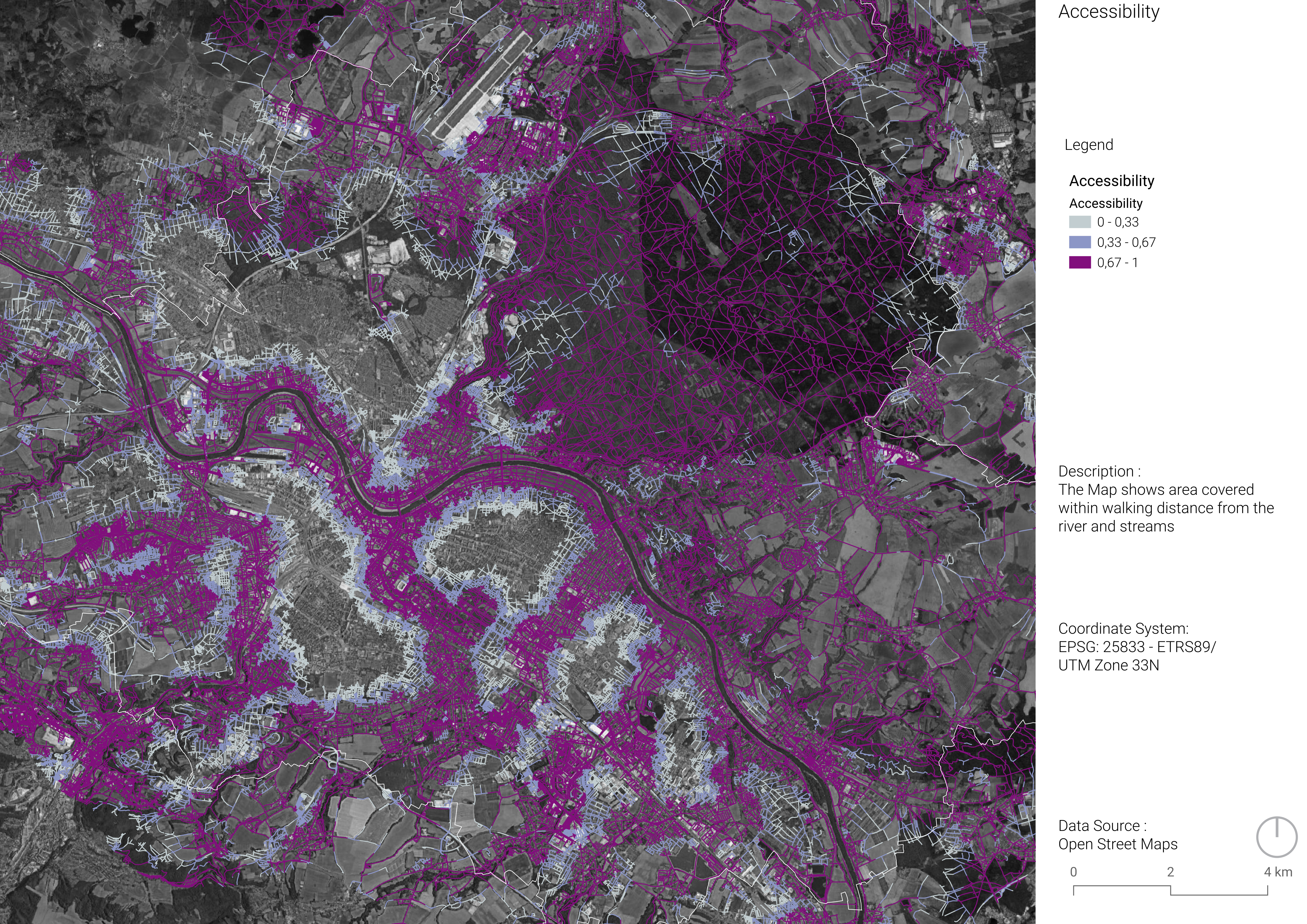
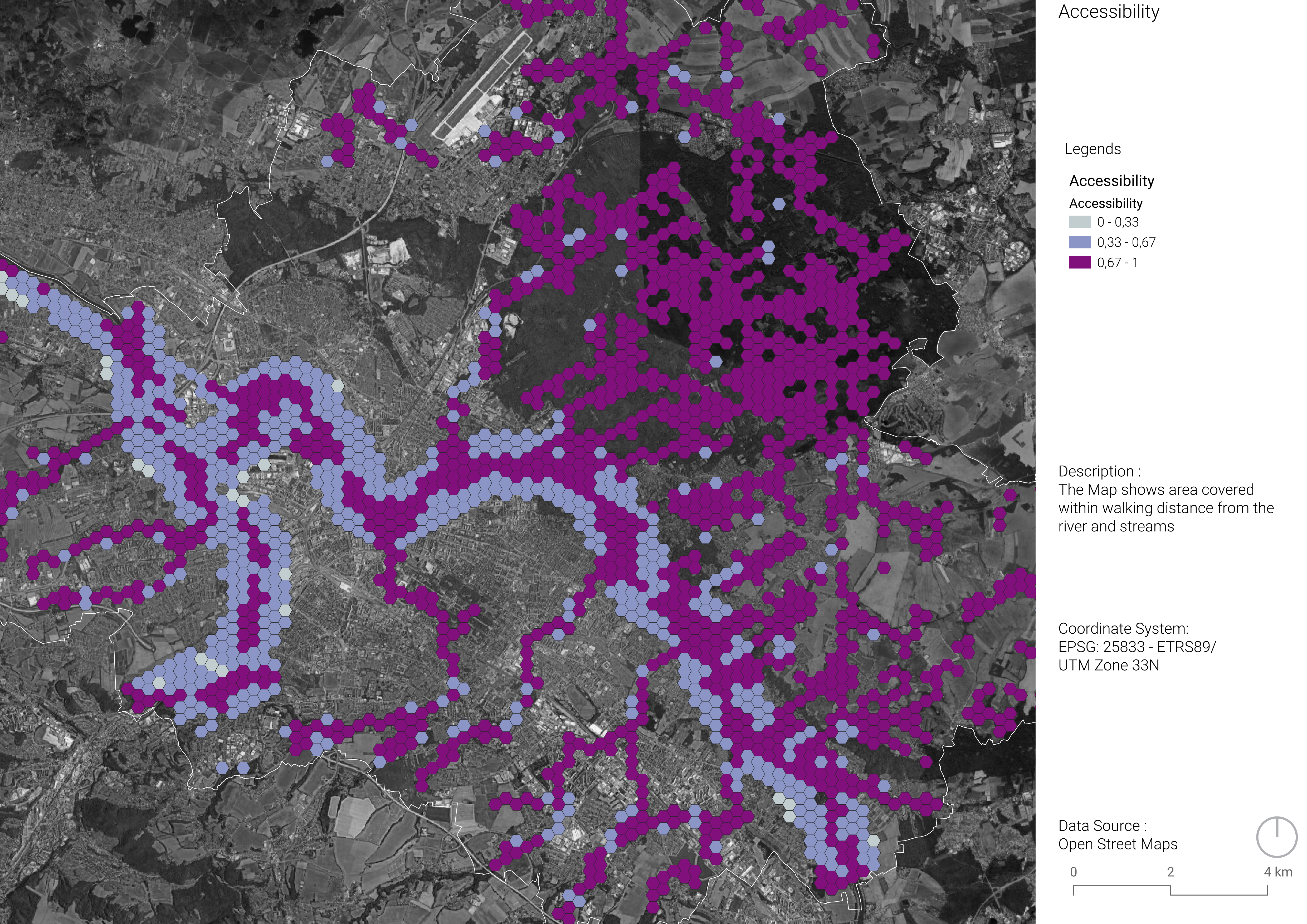
Maps Not Included in Final Results

We did an accessibility analysis to identify areas within walking distance of the streams, with steps as follows:

1. Interpolated points were generated every 500m along the stream center line and river outline.
2. Using the service area tool, we identified which areas within walking distance of interpolated points using three ranges 500m, 750, and 1000m
3. The output layers were aggregated to our the spatial units with assigned scores: 1 for areas within 500m, 0.5 for 750, and 0 for 1000m

We excluded these maps from further analysis because some spatial units had no value after aggregation.

Bernhardt, E., and M. Palmer. 2007. “Restoring Streams in an Urbanizing World.” Freshwater Biology 52: 738–51. https://doi.org/10.1111/J.1365-2427.2006.01718.X.

Dramstad, W., J. D. Olson, and R. T. Forman. 1996. Landscape Ecology Principles in Landscape Architecture and Land-Use Planning. Shearwater Books.

GovData. n.d. “EFRE 2007-2013 - Stadtteilentwicklungsprojekte - GOVData.” https://www.govdata.de/suche/daten/efre-2007-2013-stadtteilentwicklungsprojekte4de7e.

———. n.d. “Gewässersysteme - GOVData.” https://www.govdata.de/suche/daten/gewassersystemecb4ef.

———. n.d. “Web Feature Service.” https://kommisdd.dresden.de/net3/public/ogc.ashx?NodeId=1150&Service=WFS&Request=GetCapabilities.

Perrelet, K., M. Moretti, A. Dietzel, F. Altermatt, and L. M. Cook. 2024. “Engineering Blue-Green Infrastructure for and with Biodiversity in Cities.” Npj Urban Sustainability 4 (27). https://doi.org/10.1038/s42949-024-00163-y.

Riley, A. 2016. Restoring Neighborhood Streams: Planning, Design and Construction. USA: Island Press.

Riley, Ann L. 2016. Restoring Neighborhood Streams. Washington, DC: Island Press/Center for Resource Economics. https://doi.org/10.5822/978-1-61091-741-4.

Saaty, R. W. 1987. “The Analytic Hierarchy Process—What It Is and How It Is Used.” Mathematical Modelling 9 (3): 161–76. https://doi.org/10.1016/0270-0255(87)90473-8.

Scoggins, M., D. Booth, T. Fletcher, M. Fork, Ana M González, R. Hale, R. Hawley, et al. 2022. “Community-Powered Urban Stream Restoration: A Vision for Sustainable and Resilient Urban Ecosystems.” Freshwater Science 41: 404. https://doi.org/10.1086/721150.