Part 3 – Attribute Tables & Choropleth Map
Classification: Beginner GIS Analysis | Spatial Data Basics | Attribute Tables & Choropleth Mapping
Learning Level: Beginner
Time Estimate: 45 minutes
Software Required: QGIS LTR 3.44
Author: Daniele Cannatella
Overview
This exercise is the third hands-on block of the Week 1 GIS workshop, following directly on from Part 2 – Raster Import & Basemap. You will select the municipality of Vlissingen out of a province-wide density dataset (RUDIFUN), clean up its attribute table, and produce a choropleth map showing how building density changed between 2019 and 2024.
Learning Outcomes
By completing this exercise, you will be able to:
✅ Select features by attribute expression and export the selection as a new layer
✅ Delete unneeded fields from an attribute table
✅ Classify a numeric field using graduated symbology (Natural Breaks / Jenks)
✅ Calculate a new field expressing change between two years
✅ Style and export a choropleth map for sharing
Data & Software
Step 1: Select and Export the Study Area
1.1 Explore the Full Dataset
- Launch QGIS LTR 3.44
- Open the project
vlissingen-part-3.qgz - The layer
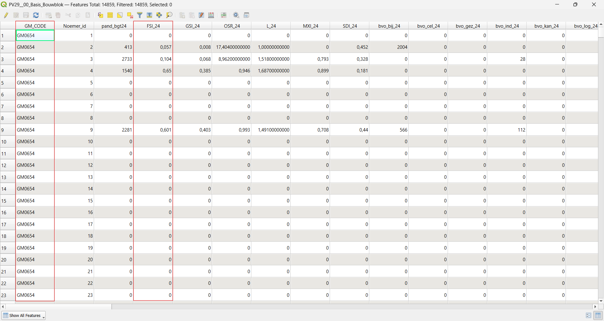
PV29__00_Basis_Bouwblokshould already be loaded, covering the whole of Zeeland - Open its Attribute Table and note the feature count and the available fields, in particular
GM_CODE(municipality code) and the FSI fields for 2019 and 2024 ([FSI_19]/[FSI_24])
Result: The attribute table lists building blocks for the entire province, not just Vlissingen.
1.2 Select Vlissingen by Expression
- Right-click the layer → Open Attribute Table
- Click Select Features Using an Expression (the ε icon)
- Enter the expression:
"GM_CODE" = 'GM0718'"GM_CODE"– the field holding the municipality code= 'GM0718'– matches rows where that code equals Vlissingen’s municipality code, written as a quoted text string
- Click Select Features
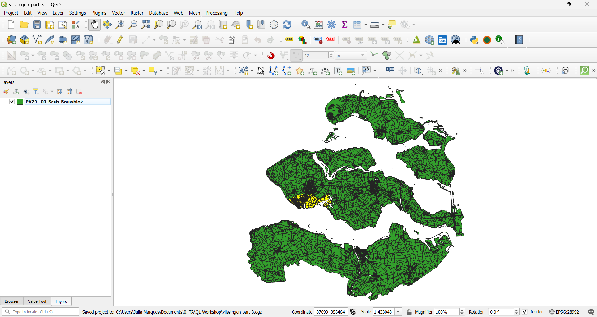
Result: Only the building blocks belonging to Vlissingen are now highlighted in yellow on the canvas and selected (highlighted) in the attribute table.
1.3 Export the Selection as a New Layer
- Right-click the layer → Export → Save Selected Features As…
- Format: GeoPackage
- Click on the three dots (besides the File name field) and navigate to the
data_outputfolder - Name:
vlissingen_rudifun - Click Save, then OK
- Add the new layer to the map if it isn’t added automatically
Step 2: Clean Up the Attribute Table
2.1 Remove Unneeded Fields
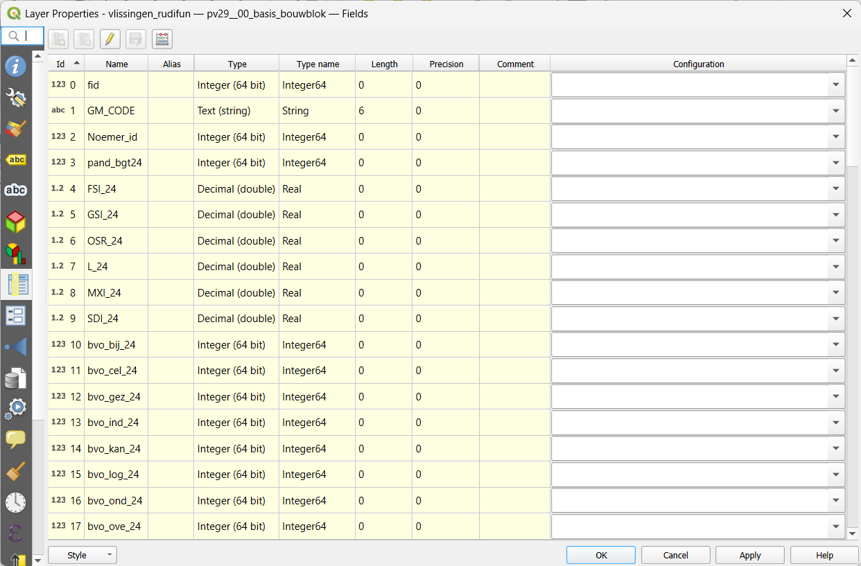
The full dataset carries many more indicators than this exercise needs. To keep the table readable, remove everything except GM_CODE and the FSI fields for 2019 and 2024.
- Right-click the
vlissingen_rudifunlayer → Properties → Fields - Click the pencil icon to toggle editing mode
- Select the fields you don’t need for this exercise, and click the Delete Field button (red X) for each
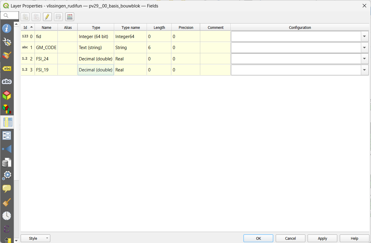
- Keep only
GM_CODE,FSI_19, andFSI_24 - Click OK to apply, then save your edits
Result: The attribute table now shows only the fields relevant to this exercise.
Step 3: Where Are the Densest Buurten in 2024?
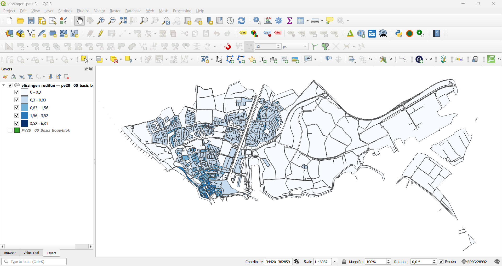
3.1 Classify by FSI 2024
- Select the
vlissingen_rudifunlayer, open Layer Styling (F7) - Change the classification type to Graduated
- Value:
FSI_24 - Classification Mode: Natural Breaks (Jenks)
- Classes: 5
- Choose a sequential colour ramp (e.g. Blues or Oranges) and click Classify, then Apply
Result: Building blocks are now shaded from low to high FSI in 2024.
Step 4: How Did Density Change Between 2019 and 2024?
4.1 Duplicate the Layer
- Right-click the
vlissingen_rudifunlayer → Duplicate Layer - Rename the copy
density_change
4.2 Filter Out Empty Blocks
Building blocks with no built floor space in 2024 aren’t meaningful for a change map, so filter them out before calculating the difference.
- Right-click
density_change→ Properties → Source - In the Provider Feature Filter box, enter:
"FSI_24" > 0- Click OK
4.3 Calculate the Change
- Open the Attribute Table for
density_change, toggle editing mode - Open Field Calculator
- Create a new field:
fsi_change(type: Decimal number) - Expression:
"FSI_24" - "FSI_19""FSI_24"– FSI value in 2024"FSI_19"– FSI value in 2019- Subtracting gives the change in FSI over the period: a positive value means the block densified, a negative value means it lost built density
- Click OK, save your edits, and toggle editing off
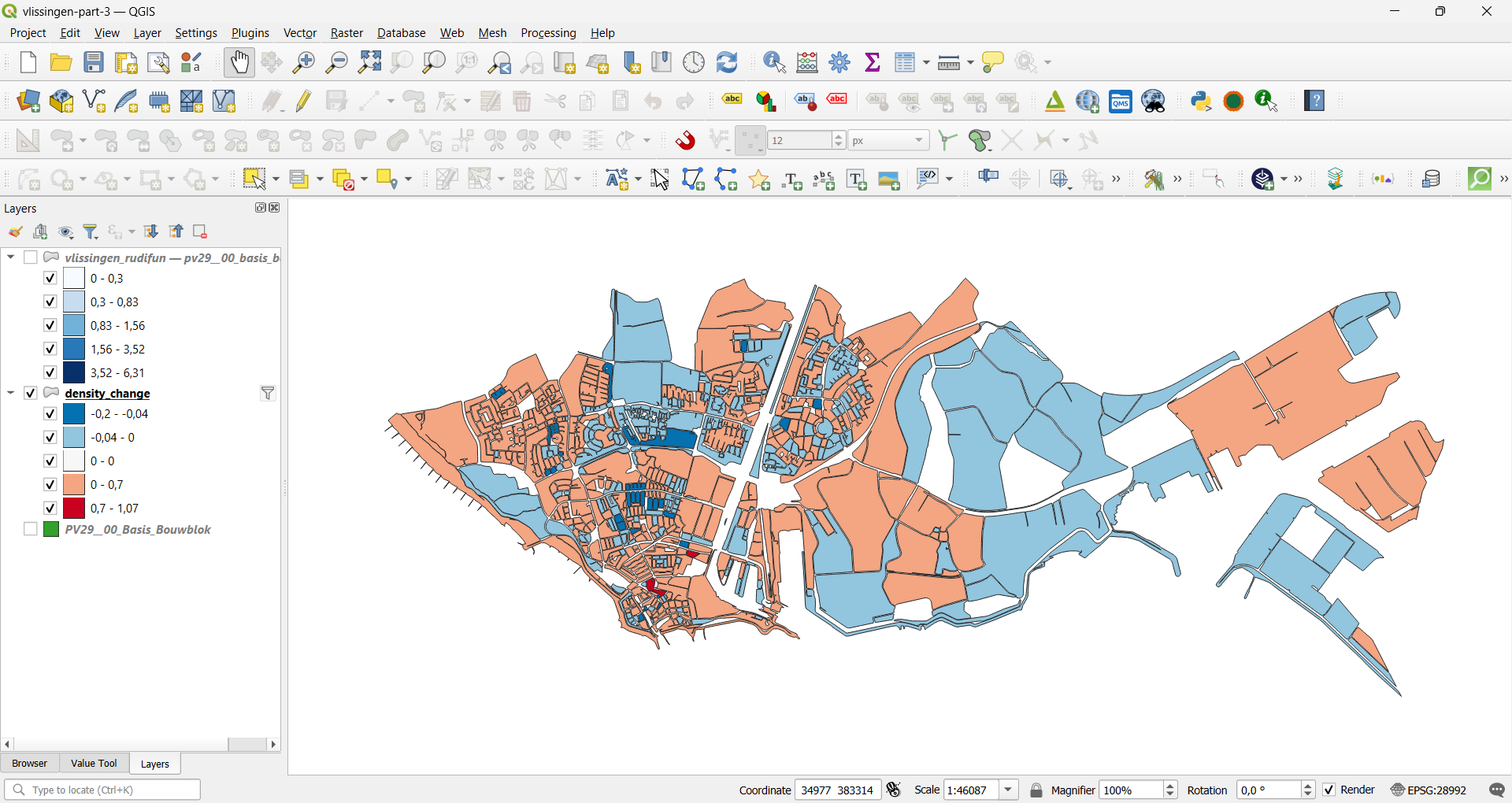
4.4 Classify the Change
- Open Layer Styling (
F7) fordensity_change - Value:
fsi_change - Choose a diverging colour ramp (e.g. RdBu or Spectral), so decreases and increases are visually distinct
- Set the classification so that 0 sits on a class break — either by choosing Natural Breaks (Jenks) and checking the generated breaks, or by manually editing a break to fall at 0
- Click Classify, then Apply
Result: Areas that densified between 2019 and 2024 appear in one colour, areas that lost density appear in the other, and the intensity of the colour shows the size of the change.
Reflection
- Why classify continuous density data into discrete classes rather than using a continuous colour ramp?
- What does the change map tell you about how Vlissingen has densified between 2019 and 2024?
- What are the limitations of comparing two snapshots in time (2019 vs. 2024) without knowing what happened in between?