Using the Data Source Manager with WFS and WMS
Duration: ~20 minutes
By the end of this exercise, you will be able to:
- Navigate and use the QGIS Data Source Manager
- Connect to and load WFS (Web Feature Service) layers from Dutch data portals
- Connect to and load WMS (Web Map Service) layers from Dutch data portals
- Understand the difference between WFS and WMS services
- Save connections for future use
- Perform basic geoprocessing operations (selection, clipping, dissolve, buffer)
- QGIS (version 3.x or higher)
- PDOK Services Plugin for QGIS
- Active internet connection
Introduction
In this exercise, you will learn how to connect to external geospatial data sources using QGIS’s Data Source Manager. You’ll work with real Dutch open data, combining different data layers to create a focused analysis area around Rotterdam and Schiedam neighbourhoods.
You will retrieve neighbourhood boundaries via WFS, perform spatial operations to create a study area, and then use this area to clip climate adaptation data. Finally, you’ll add aerial imagery via WMS to visualize your results.
This workflow demonstrates a common GIS task: defining a study area, retrieving relevant data, and preparing it for analysis.
WFS (Web Feature Service) provides access to vector data (points, lines, polygons) that you can query, style, analyze, and edit in QGIS. Think of it as downloading the actual geographic features with all their attributes. WFS is ideal when you need to perform spatial analysis or select specific features.
WMS (Web Map Service) provides access to pre-rendered map images - essentially picture tiles of maps. You cannot query individual features or access attributes, but WMS layers load quickly and are perfect for background/reference maps. Think of it as viewing a map image rather than working with the data itself.
| Feature | WFS | WMS |
|---|---|---|
| Data type | Vector (features) | Raster (images) |
| File size | Can be large | Smaller |
| Queryable | Yes | No |
| Stylable in QGIS | Yes | Limited |
| Editable | Yes | No |
| Best for | Analysis, editing, selection | Background maps, visualization |
Steps
Part 1: Setting Up Your Project and Retrieving Neighbourhood Data
Open QGIS and create a new project
Set the project CRS (Coordinate Reference System) to EPSG:28992 (Amersfoort / RD New - the Dutch standard projection)
- Go to
Project>Properties>CRS - Search for “28992” and select “Amersfoort / RD New”
- Click
OK
- Go to
Using the PDOK Services plugin, retrieve data via WFS of this dataset:
- Open the PDOK Services Plugin (look for the PDOK icon in the toolbar or go to
Web>PDOK Services Plugin) - In the plugin window, search for “CBS Wijken en Buurten 2024”
- Select the WFS option (not WMS!)
- Choose the layer:
cbs_buurten_2024(neighbourhoods) - Click to add it to your map
ImportantPlease pay attention to retrieve the correct data, as there are many buurten layers, both for WFS and WMS! What you need is a vector layer containing all 14,668 buurten (neighbourhoods) in the Netherlands. After loading, check the feature count in the layer properties to confirm you have the complete dataset.
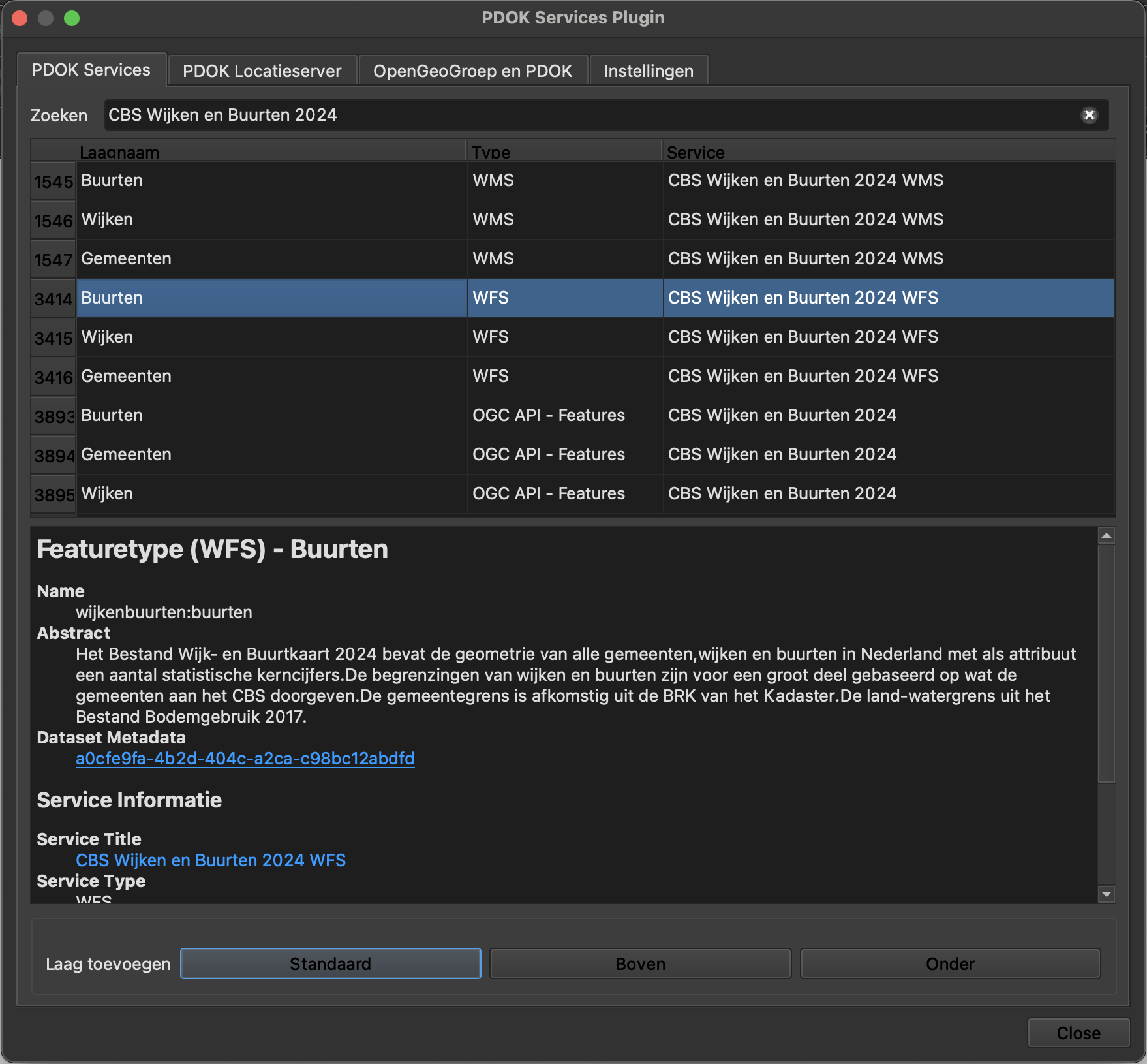
Figure 1 - PDOK Services Plugin showing CBS Buurten 2024 WFS layer ready to add - Open the PDOK Services Plugin (look for the PDOK icon in the toolbar or go to
You must now select only the 20 buurten (neighbourhoods) that meet these criteria:
- They belong to the municipalities of Rotterdam OR Schiedam (
gemeentenaam= “Rotterdam” ORgemeentenaam= “Schiedam”) AND - Their name (
buurtnaam) is one of the following: “Stationsbuurt”, “Singelkwartier”, “Natuurkundigenbuurt”, “Marconibuurt”, “Glasbuurt”, “Nieuw-Mathenesse”, “Wetenschappersbuurt”, “Newtonbuurt”, “Boylebuurt”, “Oud Mathenesse”, “Nieuw Mathenesse”, “Witte Dorp”, “Spangen”, “Tussendijken”, “Bospolder”, “Schiemond”, “Nieuwe Westen”, “Delfshaven”, “Middelland”, “Dijkzigt”
To select these neighbourhoods:
- Open the attribute table (right-click on layer >
Open Attribute Table) - Click on
Select features using an expression(the yellow icon with ε) - Enter this expression:
"gemeentenaam" IN ('Schiedam', 'Rotterdam') AND "buurtnaam" IN ('Stationsbuurt', 'Singelkwartier', 'Natuurkundigenbuurt', 'Marconibuurt', 'Glasbuurt', 'Nieuw-Mathenesse', 'Wetenschappersbuurt', 'Newtonbuurt', 'Boylebuurt', 'Oud Mathenesse', 'Nieuw Mathenesse', 'Witte Dorp', 'Spangen', 'Tussendijken', 'Bospolder', 'Schiemond', 'Nieuwe Westen', 'Delfshaven', 'Middelland', 'Dijkzigt')- Click
Select Features - Verify that 20 features are selected (shown at the top of the attribute table)
Now save the selected features:
Right-click on the layer >
Export>Save Selected Features As...Format:
GeoPackageFile name: Navigate to folder
part1_dataand name itbuurten.gpkgLayer name:
buurtenCRS:
EPSG:28992Select fields to keep:
- Click on the fields list and uncheck all columns except:
buurtnaam(name of the neighbourhood)buurtcode(code of the neighbourhood)gemeentenaam(name of the municipality)
TipYou can use the
Deselect Allbutton and then manually check only the 3 fields you want to keep.- Click on the fields list and uncheck all columns except:
Click
OKto save
Add the area column:
- Open the attribute table of the newly saved
buurtenlayer - Enable editing mode (click the pencil icon)
- Open the Field Calculator (Ctrl+I or click the abacus icon)
- Check
Create a new field - Output field name:
buurt_area - Output field type:
Decimal number (real) - Precision: 2
- In the expression box, enter:
round($area, 2) - Click
OK - Save edits (click the floppy disk icon) and disable editing mode (click the pencil icon again)
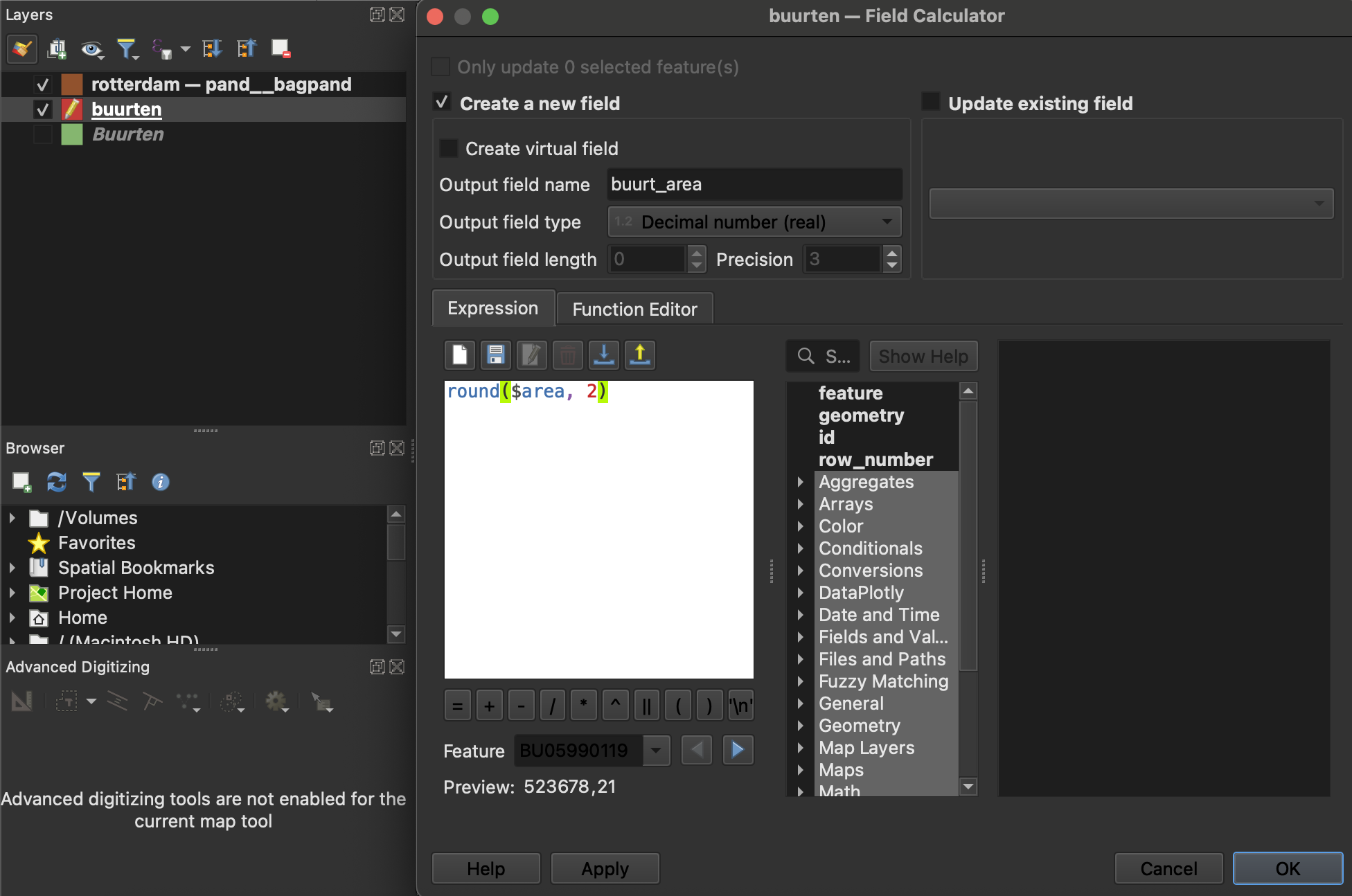
Figure 2 - Field Calculator showing the area calculation expression that rounds the area to 2 decimal places - They belong to the municipalities of Rotterdam OR Schiedam (
Dissolve the geometries of the 20 buurten into a single polygon:
- Go to
Vector>Geoprocessing Tools>Dissolve - Input layer:
buurten - Leave “Dissolve field(s)” empty (this will dissolve all features into one polygon representing the entire study area)
- Click
Run - After the temporary layer is created, right-click on it >
Export>Save Features As... - Format:
GeoPackage - File name: Select the existing
buurten.gpkgfile - Layer name:
buurten_dissolved - In the fields section, uncheck all attributes (we only need the geometry)
- Click
OK
NoteWhen unchecking all attributes, the resulting layer will have an empty attribute table containing only the feature ID (fid). This is expected - we only need the dissolved boundary geometry for further processing.
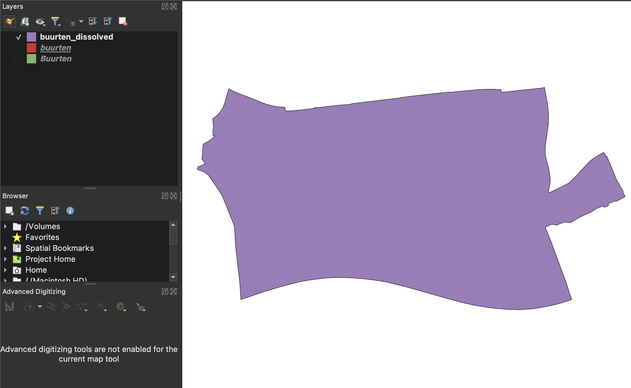
Figure 3 - Dissolved neighbourhood boundary showing all 20 neighbourhoods merged into a single polygon - Go to
Compute the bounding box (rectangular extent) of
buurten_dissolved:- Go to
Vector>Research Tools>Extract layer extent - Input layer:
buurten_dissolved - Click
Run - A temporary layer will be created showing a rectangle that encompasses your dissolved neighbourhoods
- Export this layer to the GeoPackage:
- Right-click on the extent layer >
Export>Save Features As... - File name: Select the existing
buurten.gpkg - Layer name:
bbox - Keep only columns:
minx,miny,maxx,maxy(these represent the bounding box coordinates) - Click
OK
- Right-click on the extent layer >
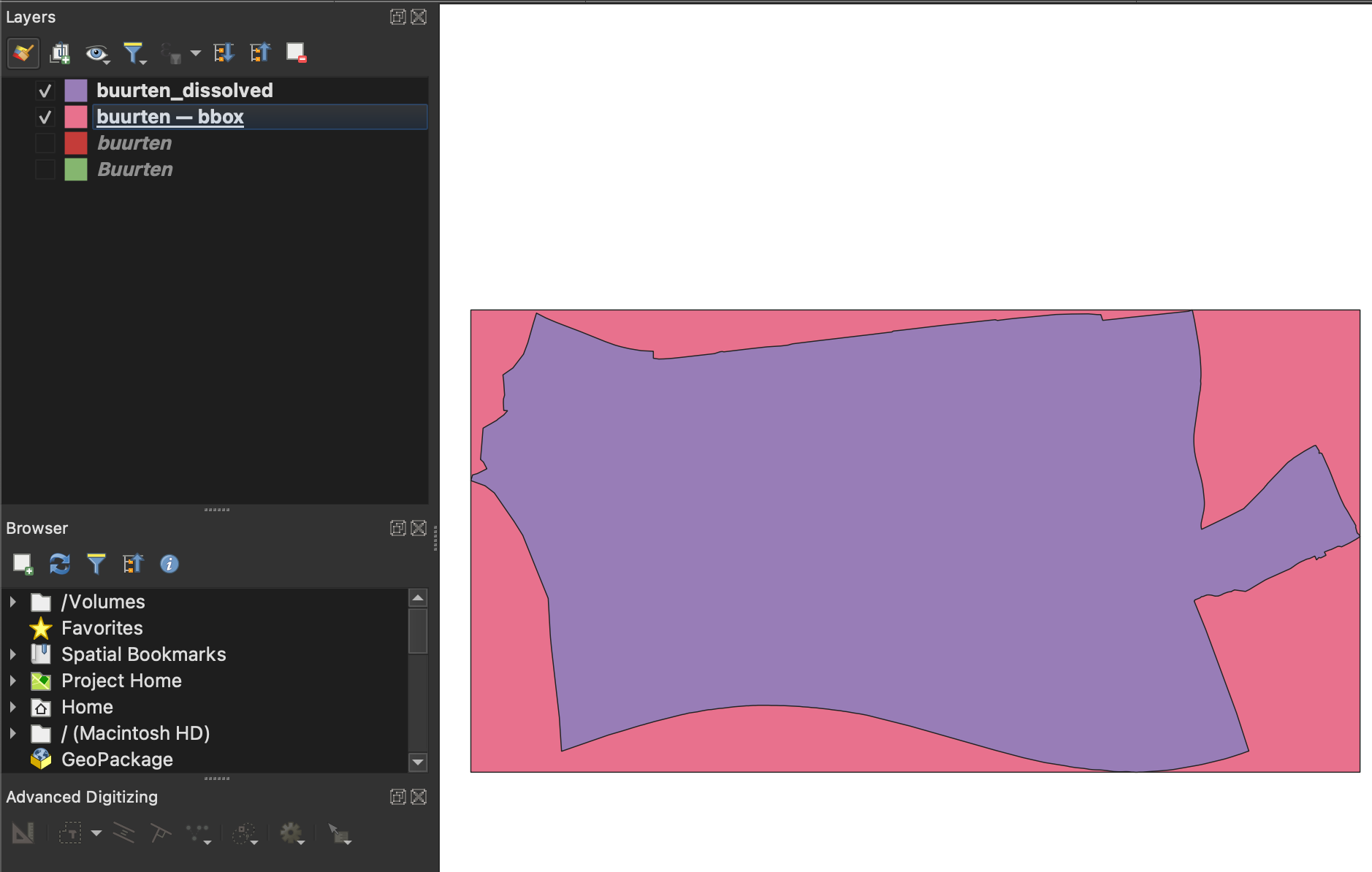
Figure 4 - Bounding box (rectangular extent) of the dissolved study area shown as a red rectangle - Go to
Finally, compute a 200 meter buffer around the bbox layer:
- Go to
Vector>Geoprocessing Tools>Buffer - Input layer:
bbox - Distance:
200(meters) - Segments: 5 (default is fine)
- End cap style:
Flat(the end cap style parameter controls how line endings are handled in the buffer) - Join style:
Miter(creates sharp corners at angles) - Miter limit: 2.0 (default)
- Click
Run - Export the result to the GeoPackage:
- Right-click on the buffered layer >
Export>Save Features As... - File name: Select the existing
buurten.gpkg - Layer name:
bbox_buffered - Uncheck all attributes in the fields section (we only need the geometry)
- Click
OK
- Right-click on the buffered layer >
Why create a buffer?The 200m buffer extends our study area slightly beyond the neighbourhood boundaries. This ensures we capture climate data for buildings that are close to but just outside the neighbourhoods, providing better context for our analysis.
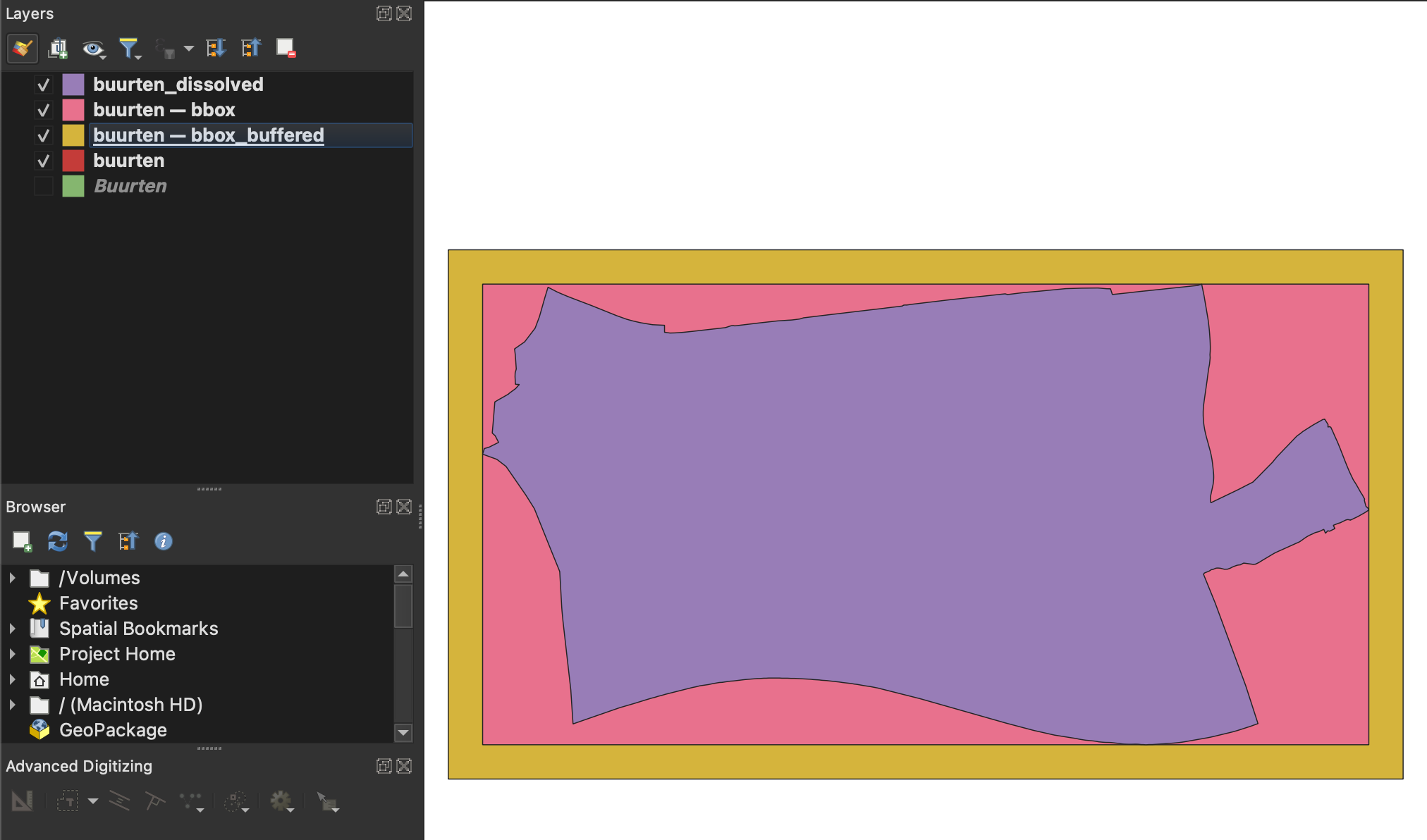
Figure 5 - 200m buffer around the bounding box, creating an expanded study area shown in green - Go to
Part 2: Connecting to WFS for Climate Adaptation Data
Open the Data Source Manager
- Click the “Open Data Source Manager” button in the toolbar, OR
- Go to
Layer>Data Source Manager, OR - Press
Ctrl+L
Select the WFS / OGC API - Features tab on the left side of the dialog
Create a new WFS connection to Zuid-Holland climate data:
- Click
Newto create a new connection - Name: Zuid-Holland Climate Adaptation
- URL:
https://geodata.zuid-holland.nl/geoserver/klimaat/wfs?service=WFS&version=2.0.0&request=GetCapabilities - Leave other settings at default
- Click
OK
- Click
Load a WFS layer:
- Select the “Zuid-Holland Climate Adaptation” connection from the dropdown and click
Connect - Wait for the available layers to load (this may take a few seconds)
- Find and select
klimaat:PANDEN_WATEROVERLAST_HITTE_GROEN(this layer contains climate adaptation data for buildings: water overlay risk, heat stress, and biodiversity indicators from 2022) - Click
Addat the bottom - Click
Closeto close the Data Source Manager
Layer name explanationPANDEN_WATEROVERLAST_HITTE_GROEN translates to “Buildings - Water Overlay, Heat, Green” and contains climate vulnerability scores for individual buildings.
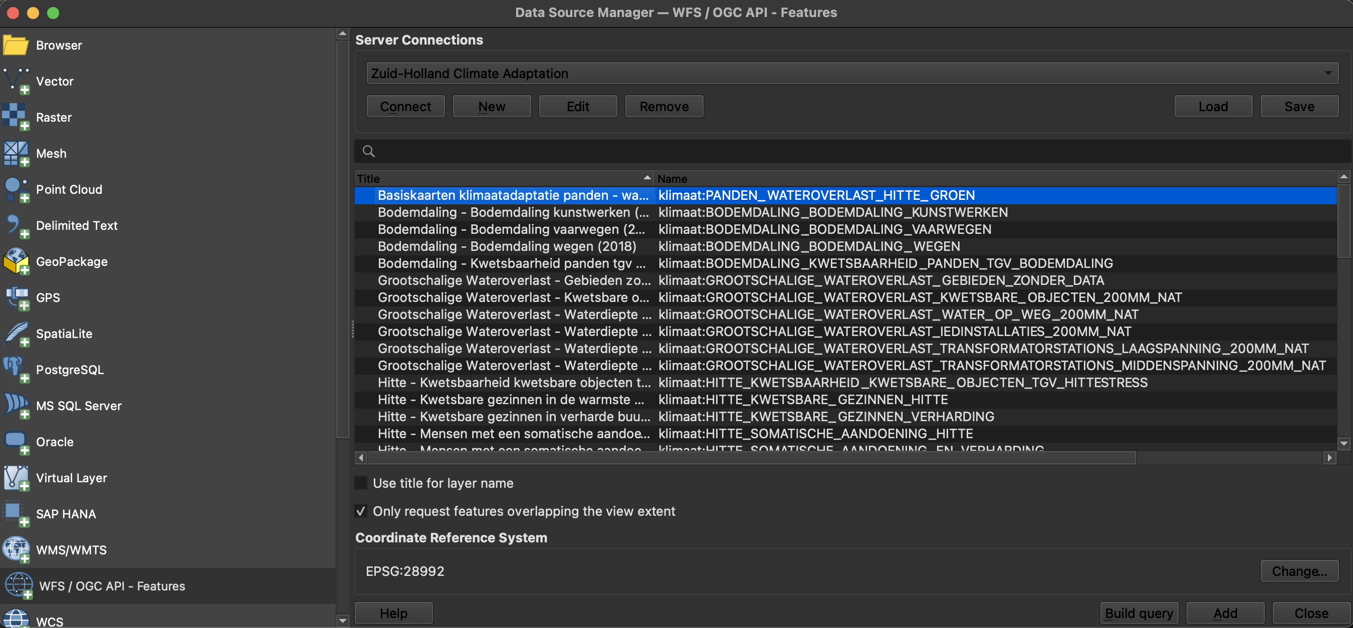
Figure 6 - Data Source Manager showing the Zuid-Holland WFS connection with available climate layers - Select the “Zuid-Holland Climate Adaptation” connection from the dropdown and click
Clip the layer to your study area:
- Go to
Vector>Geoprocessing Tools>Clip - Input layer:
klimaat:PANDEN_WATEROVERLAST_HITTE_GROEN(the climate buildings layer) - Overlay layer:
bbox_buffered - Click
Run - This will create a new temporary layer containing only the climate data within your buffered study area
- Save the clipped layer:
- Right-click on the clipped temporary layer >
Make Permanent... - Format:
GeoPackage - File name: Select or create
climate_data.gpkgin yourpart1_datafolder - Layer name:
climate_buildings_clipped - Click
OK
- Right-click on the clipped temporary layer >
- You can now remove the original (unclipped) WFS layer to improve performance
Why clip the data?The WFS layer contains data for all of Zuid-Holland province (thousands of buildings). Clipping reduces the dataset to only the buildings within our study area, making the data easier to work with and improving QGIS performance.
- Go to
Explore the layer:
- Zoom to your study area: right-click on
bbox_bufferedlayer >Zoom to Layer - Notice that buildings are vector features (polygons) you can select and query
- Open the attribute table (right-click layer >
Open Attribute Table) - Explore the climate adaptation attributes, such as:
wateroverlast_score- Water overlay/flood risk scorehittestress_score- Heat stress vulnerability score
groen_score- Green/biodiversity score
- Each building has multiple climate vulnerability indicators
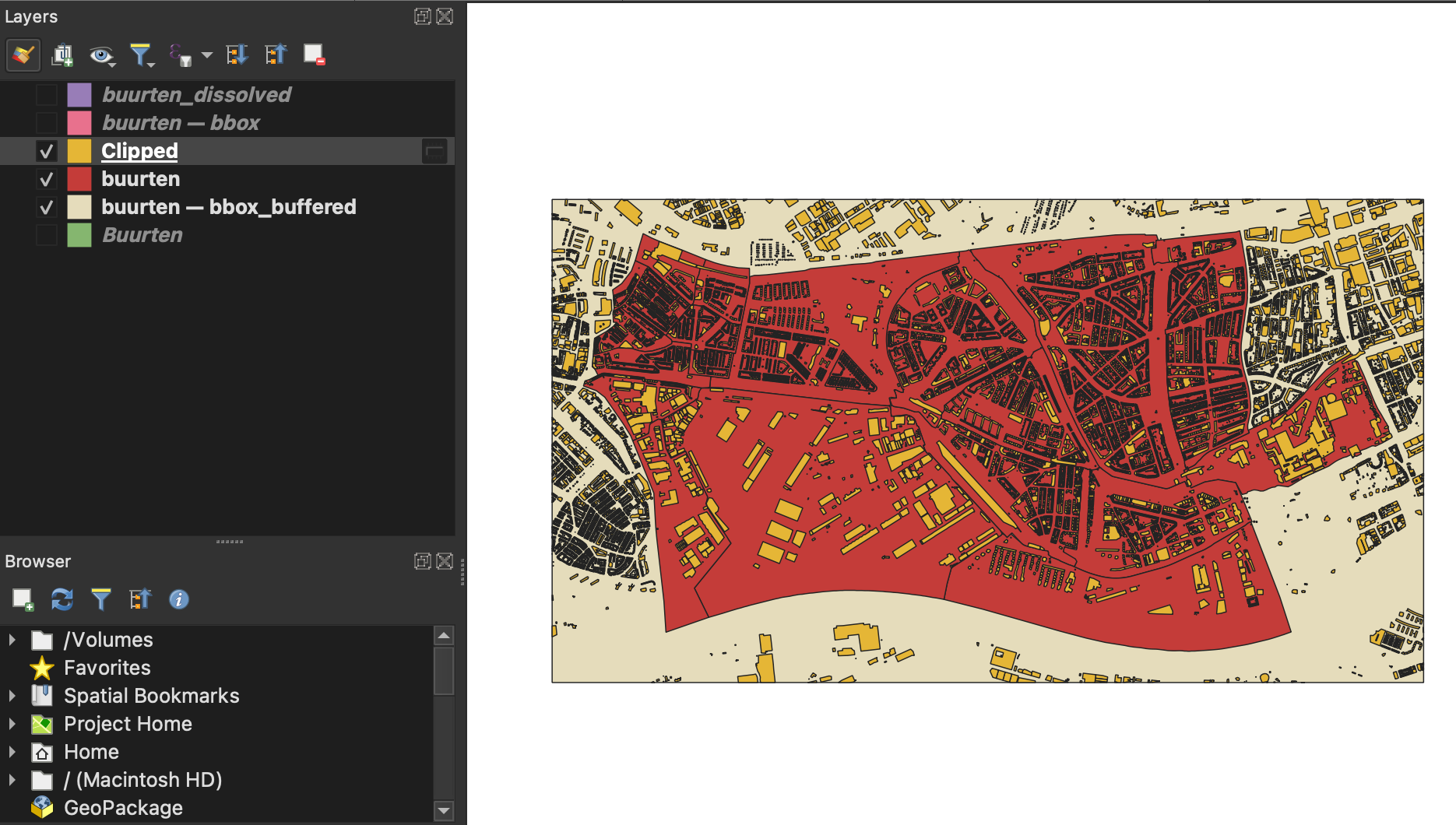
Figure 7 - Attribute table of clipped climate buildings layer showing various climate risk scores for individual buildings - Zoom to your study area: right-click on
Part 3: Connecting to WMS for Background Imagery
What is WMS? WMS provides access to pre-rendered map images - like a background map. You cannot query individual features, but it loads faster for large areas.
Before retrieving the WMS layer, you should first zoom to the study area by right-clicking the bbox_buffered layer and selecting Zoom to Layer(s). This ensures QGIS only requests tiles for your area of interest, reducing download time and file size.
Open the Data Source Manager again (
Ctrl+L)Select the WMS / WMTS tab on the left
Create a new WMS connection:
- Click
Newto create a new connection - Name: PDOK Aerial Photos
- URL:
https://service.pdok.nl/hwh/luchtfotorgb/wmts/v1_0?request=GetCapabilities&service=wmts - Leave other settings at default
- Click
OK
- Click
Load a WMTS layer:
- Select the “PDOK Aerial Photos” connection and click
Connect - Wait for available layers to load
- Find and select
Luchtfoto 2025 Ortho 25cm RGB(current high-resolution 25cm aerial photos) - Important: In the “Coordinate Reference System” section, select
EPSG:28992from the dropdown - Click
Add - Click
Close
WMTS vs WMSWMTS (Web Map Tile Service) is a variant of WMS that serves pre-generated map tiles, making it faster for viewing at standard zoom levels.
- Select the “PDOK Aerial Photos” connection and click
Save a local copy of the orthophoto:
This step saves the aerial imagery as a permanent file that you can use offline and in future projects.
- Select the orthophoto layer in the Layers panel
- Right-click on it and choose
Export>Save As...
In the resulting dialog, set the following parameters:
- Output mode:
Rendered image(this saves what you see on screen) - Format:
GeoTIFF - Important: Uncheck “Create VRT” (we want a standard GeoTIFF file, not a virtual raster)
- File name: Click
...and navigate to the\part1_data\rasterfolder (create it if it doesn’t exist)- Name the file:
ortho_25cm.tif
- Name the file:
- CRS:
EPSG:28992(should already be set) - Extent: Click the dropdown and select
Calculate from Layer>bbox_buffered- This ensures you only save imagery for your study area
- Resolution:
- Horizontal:
0.25(meters per pixel) - Vertical:
0.25(meters per pixel)
- Horizontal:
- Click
OKto start the export - Wait for the export to complete (this may take 1-2 minutes depending on the area size)
- The saved GeoTIFF will be automatically added to your map
Understanding ResolutionThe 0.25m resolution means each pixel in the saved image represents 25cm × 25cm on the ground. This matches the native resolution of the PDOK aerial photos, ensuring no quality loss.
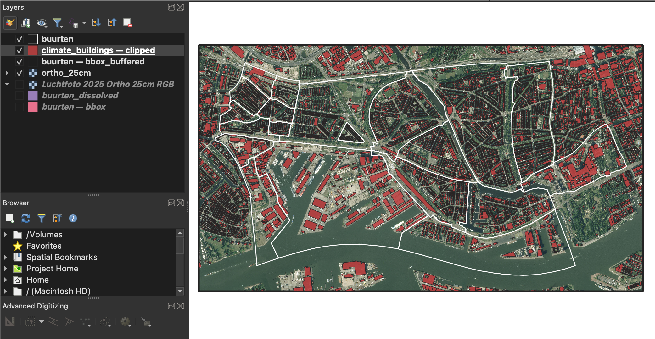
Figure 8 - Export Raster dialog showing proper settings for saving the aerial photo with correct extent and resolution Arrange your layers for optimal visualization:
- In the Layers panel, drag layers to arrange them in this order from top to bottom:
buurten(neighbourhood boundaries - should be visible as outlines)climate_buildings_clipped(climate data polygons)bbox_buffered(buffer outline - optional, can be hidden)ortho_25cm.tifor the WMTS aerial photo layer (at the bottom as background)
Style adjustments:
- Neighbourhood boundaries (
buurten):- Right-click >
Properties>Symbology - Set fill to “Simple fill”
- Fill style:
No Brush(transparent) - Stroke color: Red or dark blue
- Stroke width: 0.5 - 1.0 mm
- Right-click >
- Climate buildings:
- Adjust transparency: Right-click >
Properties>Symbology>Layer Renderingtab - Set opacity to 70-80% so you can see the aerial photo underneath
- Optionally, style by climate scores using categorized or graduated symbology
- Adjust transparency: Right-click >

Figure 9 - Final map view showing neighbourhood boundaries, climate data, and aerial imagery properly layered with appropriate transparency - In the Layers panel, drag layers to arrange them in this order from top to bottom:
Recap
What you’ve learned:
- The Data Source Manager is your central hub for connecting to external data sources in QGIS
- WFS provides vector data that you can style, query, and analyze - great for operational data and spatial analysis
- WMS/WMTS provides raster map images - great for background maps and visualization
- How to use the PDOK Services Plugin to easily access Dutch open geospatial data
- Basic geoprocessing workflows: selection, dissolve, buffer, clip, and extract extent operations
- How to organize and save multiple layers in a GeoPackage for efficient data management
- How to export and save WMS/WMTS imagery as permanent GeoTIFF files
- Dutch PDOK (Publieke Dienstverlening Op de Kaart) offers free, reliable geospatial web services
- Provincial and municipal data portals (like Zuid-Holland) provide specialized datasets
- Saved connections can be reused in future projects
Key differences between WFS and WMS:
| Feature | WFS | WMS/WMTS |
|---|---|---|
| Data type | Vector (features) | Raster (images) |
| File size | Can be large | Smaller |
| Queryable | Yes | No |
| Stylable in QGIS | Yes | Limited |
| Best for | Analysis, editing | Background maps |
Useful Dutch Data Portals:
- PDOK: https://www.pdok.nl/ (national geospatial infrastructure)
- Data.overheid.nl: Open data from Dutch government
- Nationaal Georegister: https://www.nationaalgeoregister.nl/ (search for geospatial services)
- Most Dutch provinces and municipalities also offer their own WFS/WMS services
Extension Activities (Optional)
- Explore other PDOK services at https://www.pdok.nl/datasets
- Try filtering WFS layers using the Data Source Manager’s “SQL” or “Filter” options before loading
- Analyze the climate adaptation scores in your selected Rotterdam and Schiedam neighbourhoods
- Compare different neighbourhoods’ vulnerability to heat, water, or biodiversity loss using statistics
- Add the RIVM Energy Labels WMS (
https://data.rivm.nl/geo/nl/wms?request=GetCapabilities, layerrvo_energielabels) to see building energy performance ratings - Create a styled thematic map showing the relationship between neighbourhood characteristics and climate risks
- Calculate summary statistics (mean, max, min) of climate scores by neighbourhood