Part 1 – Vector Import & Basemap
Classification: Beginner GIS Analysis | Spatial Data Basics | Vector Import
Learning Level: Beginner
Time Estimate: 30 minutes
Software Required: QGIS LTR 3.44, QuickMapServices (QMS) plugin
Authors: Daniele Cannatella and Julia Fossa Marques
Overview
This exercise is the first hands-on block of the Week 1 GIS workshop. You will import two vector layers — a land use layer and a neighbourhood boundary layer — for the municipality of Vlissingen, style them, add an OpenStreetMap basemap, and produce a basemap screenshot for the Miro board.
Learning Outcomes
By completing this exercise, you will be able to:
✅ Import vector layers into QGIS from the Browser Panel
✅ Check a layer’s feature count and coordinate reference system (CRS)
✅ Add an OpenStreetMap basemap using the QuickMapServices plugin
✅ Style a categorical vector layer by attribute
✅ Export a styled map view as an image for sharing
Data & Software
Step 1: Import and Explore the Data
1.1 Open the Project and Import the Layers
- Launch QGIS LTR 3.44
- Open the project
vlissingen.qgz - From the Browser Panel, import the land use layer
bbg.gpkg - From the Browser Panel, import the neighbourhood boundary layer
vlissingen_neighbourhoods.gpkg
Result: Both the bbg and vlissingen_neighbourhoods layers should now appear in the Layers Panel and draw on the canvas over Vlissingen.
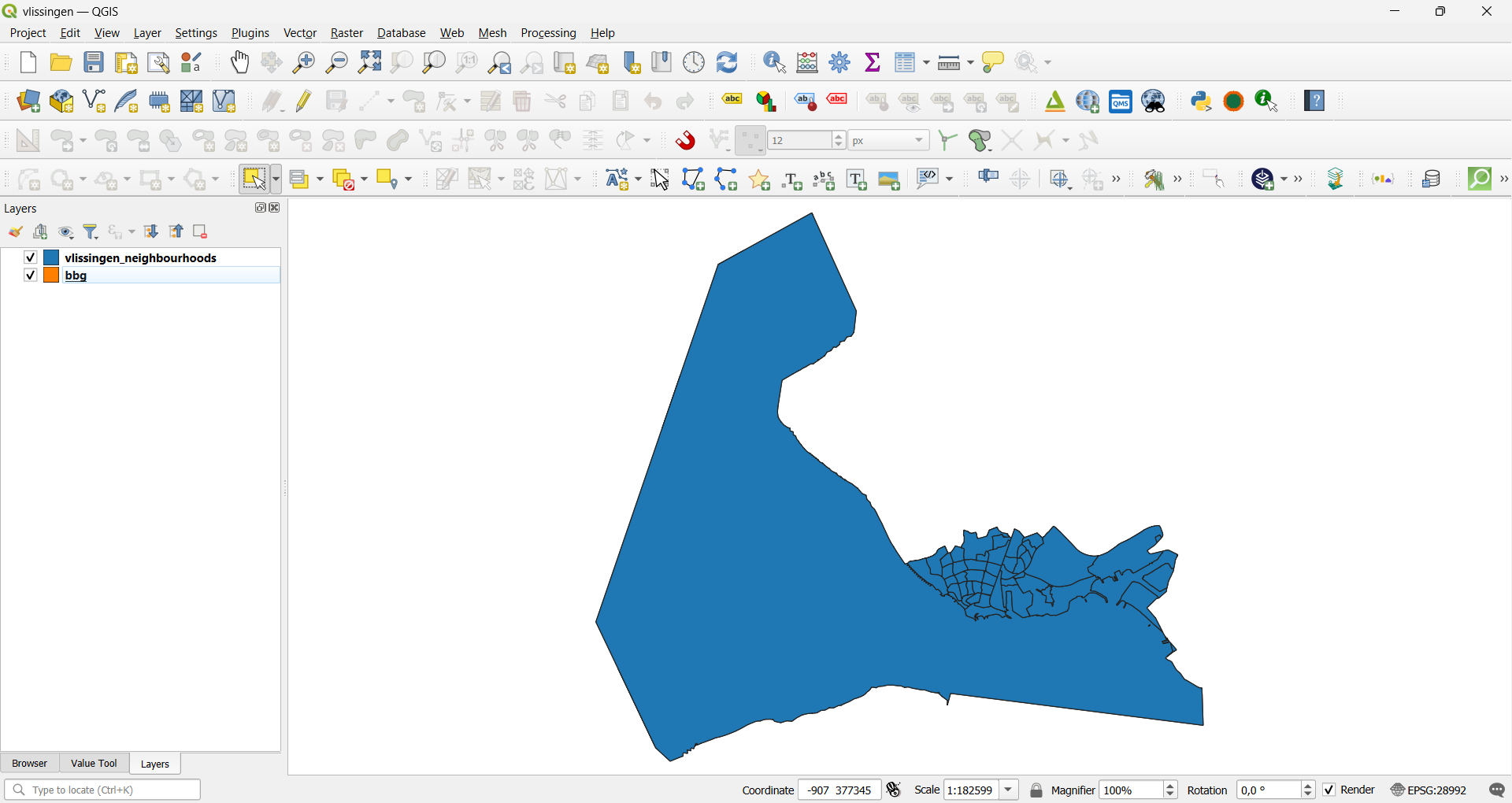
1.2 Explore the Layers
Step 2: Add an OSM Basemap
- Install the QuickMapServices (QMS) plugin if not already installed: Plugins → Manage and Install Plugins, search for
QuickMapServices, click Install Plugin - Go to Web → QuickMapServices → OSM → OSM Standard to add an OpenStreetMap basemap
- Drag the basemap layer to the bottom of the Layers Panel, below
bbgandvlissingen_neighbourhoods
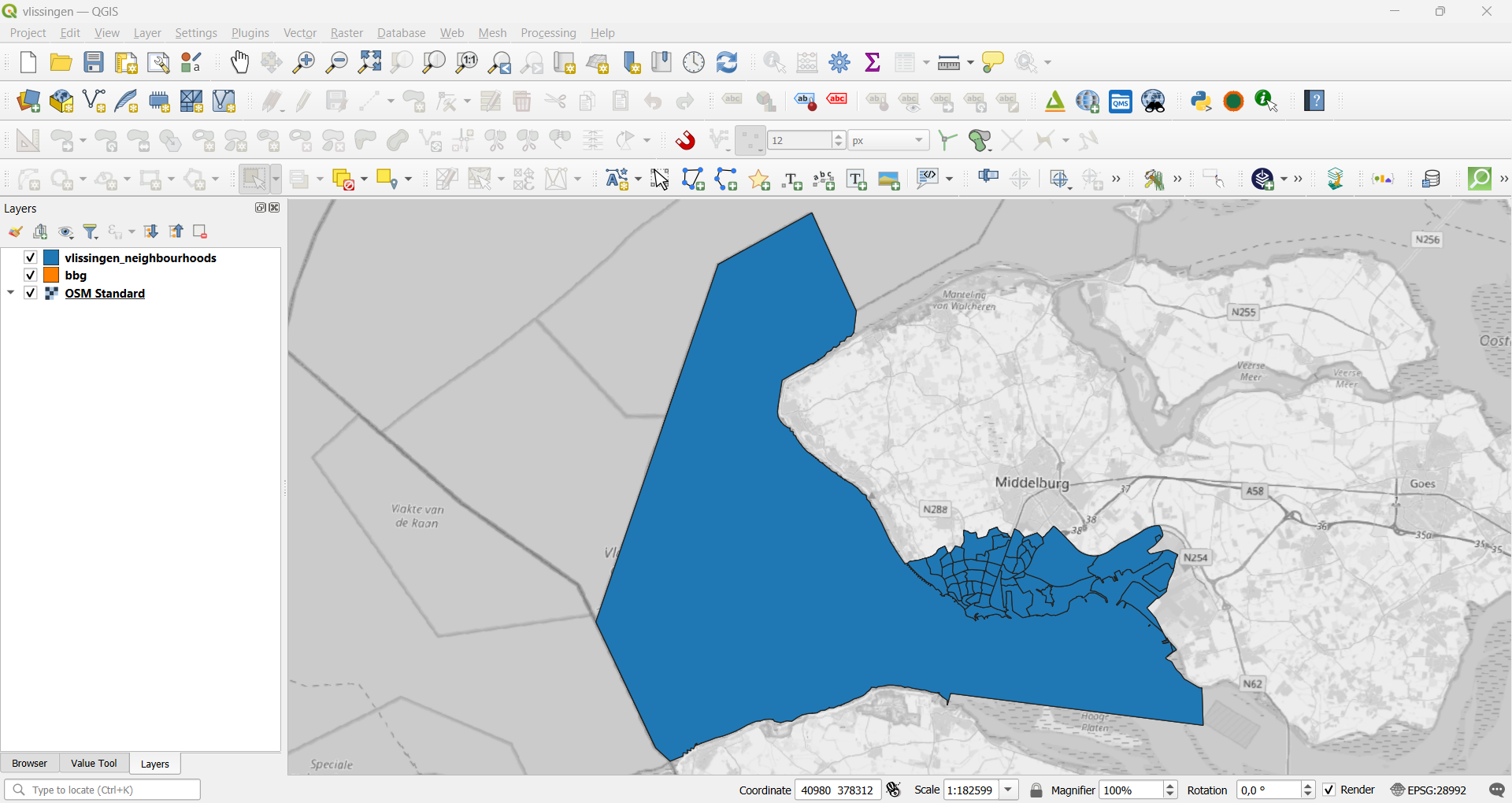
Step 3: Style the Layers
3.1 Style the Land Use Layer by Category
- Select the
bbglayer, open Layer Styling (F7) - Change the symbology to Categorized
- Value:
categorie - Choose a colour ramp and click Classify
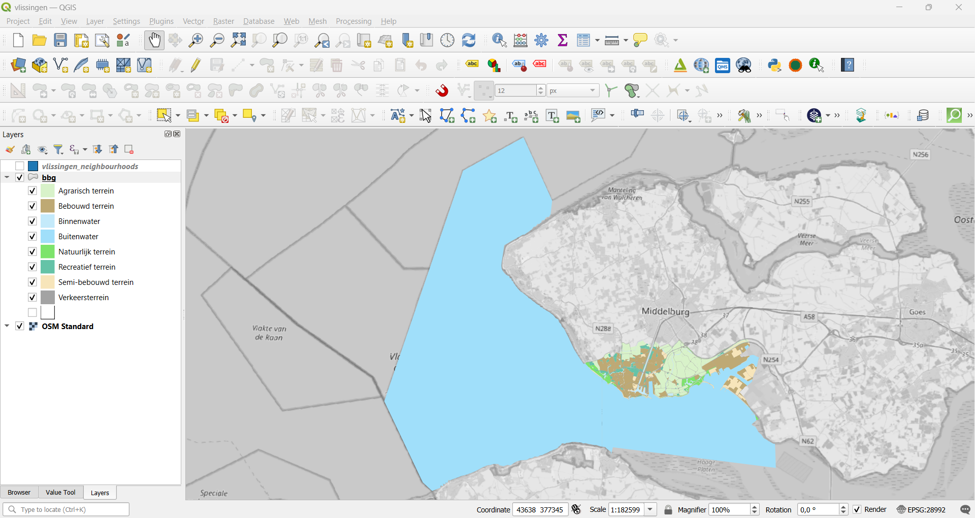
3.2 Style the Neighbourhood Boundaries
Select the
vlissingen_neighbourhoodslayer, open Layer Styling (F7)Set the symbol fill to No Fill and choose a visible outline colour/width, so boundaries are readable on top of the land use layer
Zoom in to the land area (using the mouse scroll or clicking on the magnifying glass icon)
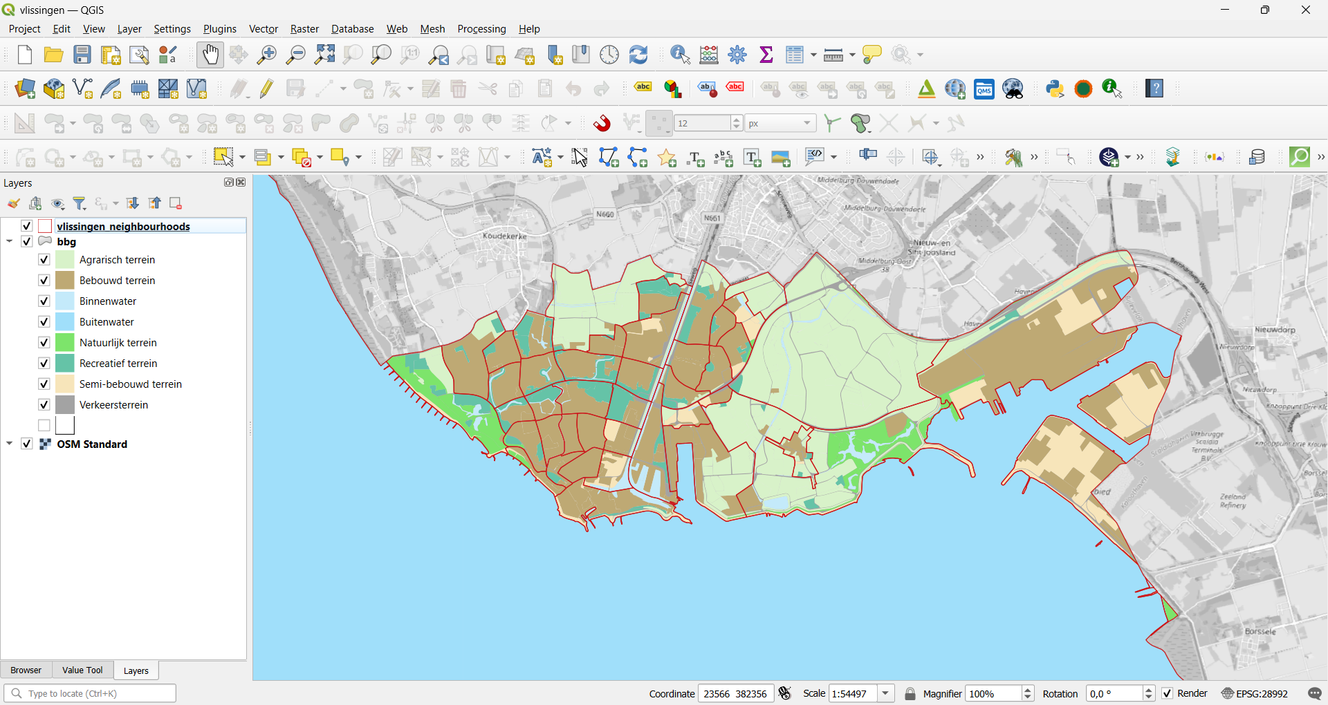
Reflection
- What did you choose to highlight in your map, and how did your styling choices support that?
- How does adding the neighbourhood boundaries change how you read the land use pattern?